


Introduction to SEP statistical models
Statistical models built for the description of the
SEP event environment aim to associate estimated characteristic values of the events with a given probability of occurrence at a given period of known or predicted solar activity level.
Their outputs are dependent upon the collected raw data and the subsequent processing of the flux time series. It is evident that the quality (e.g. noise, data gaps, and calibration errors), the time span of the data as well as the definition used for the creation of
SEP event lists, are some of the critical issues [1,2] in the development of a radiation environment statistical model. The prediction of a SEP environment generally requires the combination of two probability density function (pdf) distributions; one for the characteristic quantity of interest (fluence, peak flux or event duration) and another for the waiting time (or frequency) of the events.
SEPEM includes a suite of standard models, such as the Jet Propulsion Laboratory (JPL) [3-5] or the Emission of Solar Proton (ESP) models [6-8], as well as new methods that involve direct sampling of event waiting times [9].
In what follows, we briefly present the standard distribution functions that are used for the statistical description of SEP event environments. The random sampling of their cumulative density function (cdf) is used for the extraction of characteristic values of the modeled events. Subsequently, the different methods that are applied in SEPEM for the combinations of the distributions are discussed.
Fluence and peak flux distributions of SEP events
Quantities of SEPs are measured in counts but given in terms of fluxes which account for different instrument geometries and necessary correction factors. The definition for differential fluxes standard in SEPEM is number of particles arriving over a specified area in a certain time period at a specified energy. The peaks are the highest values over the course of an SEP event averaged over the sampling time often determined by the instrument [standard units are cm-2s-1sr-1MeV-1]. The fluence (or integral flux) is the flux summed over the complete duration of the event [standard units are cm-2sr-1MeV-1].
To model the SEP event radiation environment SEPEM includes fitting of the lognormal, the truncated power law and the cut-off power law distributions to fluences and peak fluxes of SEP events.
The Lognormal distribution
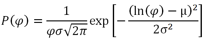
The probability density function (pdf) of the lognormal distribution is given by the following equation:
| (1) |
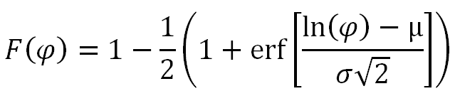
Here φ is the event fluence, μ the mean value and σ the standard deviation of the natural logarithm of the event fluences. The event fluences in the JPL models have been fitted with the lognormal distribution [3-5]. The cdf of the lognormal distribution is given by:
| (2) |
where
F(φ) is the likelihood of an event having fluence above φ. In the modelling the cdf is used and randomly sampled to get a fluence value for each event. Note that the lognormal distribution fails to fit the entire range of the data and particularly the lowest fluences. However, the contribution of these small events to the total cumulative fluence is negligible. In addition, the distribution has provided the best fit to the total yearly fluence when considering only those years during 7-year solar maximum [6]. Note that the lognormal distribution as used in the JPL model [3-5] is actually the normal distribution applied to the log
10 of the event fluences or peak fluxes and this was applied for functions on the SEPEM system. Although ultimately whether the natural logarithm or the log
10 is used in the calculation makes no difference to the model output it will make a difference when comparing distribution parameters with others previously published.
The truncated power law
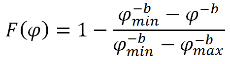
A truncated form of the power law has been successfully used to fit distributions of peak fluxes of events [7] and of the event fluences [8]. The cdf of the truncated power law is given by:
| (3) |
and provides the likelihood for a single event fluence (peak flux) to exceed the value
φ. The minimum event fluence (peak flux)
φmin is an input parameter defined by the event list while the exponent of the power law,
b, and the maximum event fluence (peak flux)
φmax are numerically determined through the fitting procedure. The truncated power law distribution has been used up to now only for the worst cases (of peak flux and fluence) but SEPEM allows the user to utilise it for the modelling of the cumulative mission fluence as well [9].
The cut-off power law
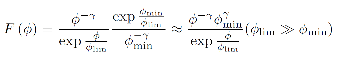
The cut-off power law as used in the MSU model [13] displays a power law behaviour until the high intensity end of the distribution where an exponential function determines the deviation from the power law. This function is given by:
| (3) |
where b is the exponent of the power law and φco is the cut-off parameter, if φ is << φco then power law behaviour is recovered. Unlike the truncated power law, there is no maximum value but a reduction in the probability of an event for φ > φco compared to a power law which becomes greater with greater φ.
Time distributions of SEP events
The Poisson, the time-dependent Poisson and Lévy distributions have been used to fit the waiting time and duration distributions of SEP events [14]. The inverse Fourier transforms of these distributions provide the pdf of the event frequency. A brief description follows.
The Poisson, the time-dependent Poisson and Lévy distributions have been used to fit the waiting time distributions of SEP events. The inverse Fourier transforms of these distributions provide the pdf of the event frequency. A brief description follows.
The Poisson distribution
A Poisson process requires the events to be time-independent and with a steady mean rate of occurrence. Therefore the Poisson distribution is applicable in SEP environment models only for solar active years, within which most of the SEP event fluence is contained and the event rate can be considered approximately steady [3]. The expression of a Poisson process in the time domain is given by the pdf of the exponential distribution:
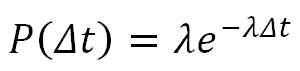
| (4) |
Integration of the latter provides the following cdf:
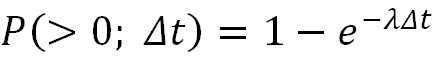
| (5) |
which defines the likelihood
P(>0;Δt) of observing at least one event in time
Δt.
The time-dependent Poisson distribution
The time-dependent Poisson distribution—in contrast to the time-steady Poisson—describes processes with varying (mean) event rate that are locally Poissonian. As a consequence, it allows the modelling of complete solar periods including quiet years.
The waiting time pdf of the time-dependent Poisson distribution has been applied for the modelling of solar flares and CMEs [10], and is given by
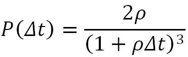
| (6) |
Equation (6) follows a power behavior at high waiting times but predicts fewer events at low waiting times. Integration of equation (6) provides the cdf of the waiting time distribution,
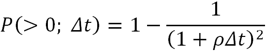
| (7) |
which defines the likelihood
P(>0;Δt) of an occurrence at least one event in time
Δt. The latter can be sampled to find a random waiting time.
The Lévy distribution
The Poisson distributions cannot treat events that are inter-dependent in time. In contrast, Lévy processes allow both for short-term memory (over consecutive events) as well as for long-term variations of the activity in the process. The transform of the symmetric Lévy distribution into the time domain provides the following pdf:
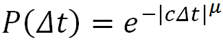
| (8) |
The use of the Lévy distribution for the modelling of SEP events was first suggested by Gabriel and Patrick [11].
P(Δt) is the probability density for waiting time
Δt over a specified time period, the exponent
μ lies in the range [0,2] and
c is a scaling parameter. The integration of the pdf leads to the following cdf:
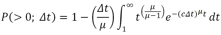
| (9) |
from which a random waiting time may be sampled. It should be stressed that, unlike the Poisson distribution, the Fourier transform from the time domain to frequency domain is not straightforward and requires a non-trivial numerical integration [12].
Methods for the combinations of distributions
The generation of a prediction of SEP event environment generally requires the combination of two pdf's; one for the characteristic quantity of interest (fluence, peak flux or event duration) and another for the waiting time (or frequency) of the events. In SEPEM the following combination methods have been utilized in the statistical tools provided.
Monte Carlo method
This method is used to combine event frequency pdf and SEP event characteristic in a similar manner as in JPL models [3-5]. A pdf for the event frequency is generated and a number of runs proportional to the density of each event frequency is defined. The characteristic values of SEP events are randomly generated for the required number of events in each run using the constructed pdf. The number of the Monte Carlo (MC) runs for the calculation of the confidence level of each quantity is sufficiently large to ensure smoothness in the statistical curves. However, for the creation of a model for the likely time duration spent above a flux threshold the MC method is not appropriate since the event frequency pdf assumes that the SEP events are point-like in time and that a subsequent event may occur immediately.
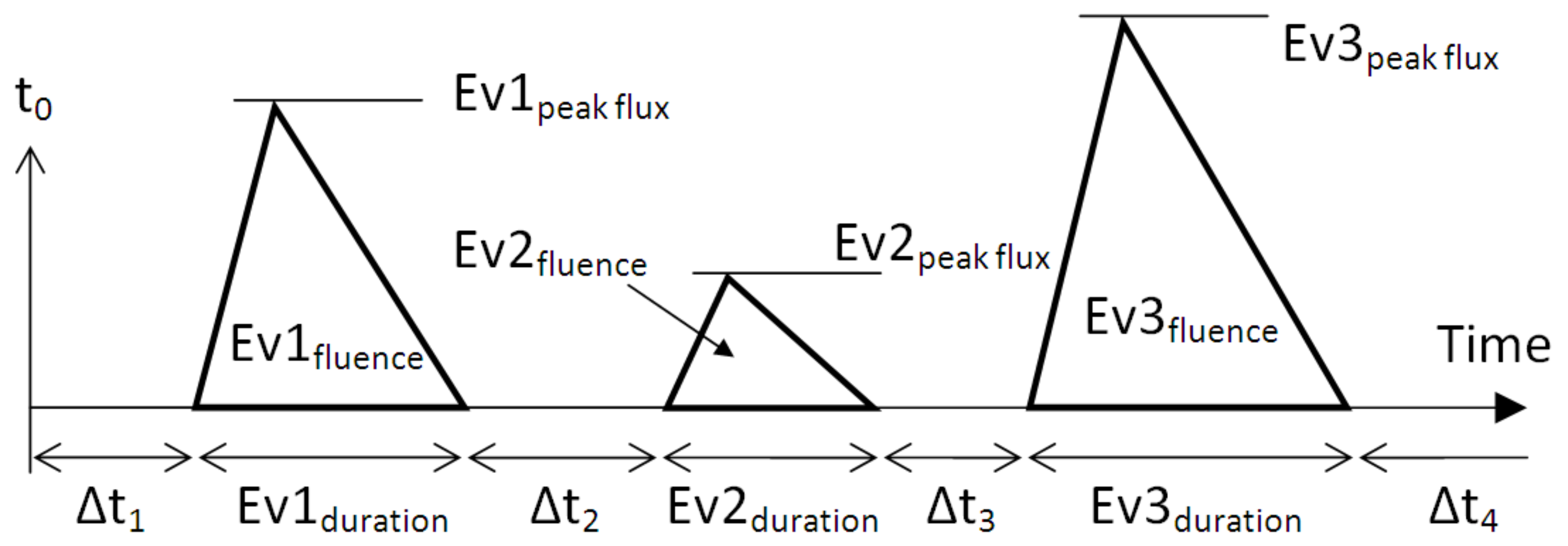
Virtual timelines method
This method is used to intersperse SEP event characteristics and waiting times [9]. After each waiting time, defined from the end of one event to the beginning of the next, a fluence (or peak flux) for the coming event is generated. This procedure creates a virtual timeline of associated cumulative and/or maximum values of the selected characteristic. In the case of cumulative fluence models the generated value is added to the running total, while in the case of worst-case event fluence (peak flux) the generated value replaces the running worst-case when the latter is smaller. The virtual timelines method accounts for the significant durations of SEP events by use of a semi-empirial regression to determine a andom event duration factoring in the fluence (peak flux). The results do not vary significantly compared to those derived by the MC method when the same or reciprocal distributions are used. However, the virtual timelines method can be applied for the creation of event duration statistical models and can allow for an altering of the orbit and/or solar activity level over the course of the planned mission. A cartoon illustrating this modelling method is shown below:
| (10) |
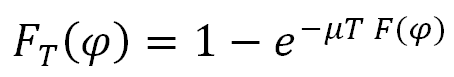
Analytical worst case ESP method
When the frequency of the events follow a Poisson distribution, and the distribution of a characteristic (peak flux, fluence) follows a power law, the likelihood of the worst case characteristic can be expressed analytically by the following equation [7]:
| (10) |
Here
FT(φ) is the likelihood of the worst case event peak flux (or fluence) to be greater that φ in time period
T,
F(φ) is the initial cumulative distribution (or the likelihood of a single event exceeding the value φ) and
μT is the average number of events for
T.
Time Period (Mission Length)
The time period parameter dictates which part of the solar cycle is considered, active years are defined as being from 2.5 years before to 4.5 years after the maximum smoothed monthly sunspot number for each solar cycle.
Total time period
Choosing Total time period ignores the variance of SEP event frequency over the course of a solar cycle. If the mission designer does not know when a mission will be launched they are advised to be conservative and select the Active years only option instead. This option is mainly for comparison purposes only.
Active years only
Choosing Active years only assumes that the mission will experience only periods of high activity when it is known that the SEP event frequency is higher. The division of the 11-year solar cycle into 4 quiet years and 7 active was suggested by Feyman et al. [3]. When performing the analysis only the fluences, peak fluxes, durations and waiting times between those events during the active years
of the sample data are used. This option should be selected if a mission is to occur only during active years or the user does not know in which phase of the solar cycle the mission launch date will be.
Quiet years only
In 2005 and 2006 there were several large SEP events outside of the solar active years prompting modellers to consider whether solar quiet years should be considered. It is known that the SEP event frequency during these times is lower but it is not established whether the event fluences (peak fluxes) are smaller or not. When selecting this option the analysis uses the mean SEP event frequency for the quiet periods in the selected event list to determine an event frequency distribution. There are insufficient events to do a good fit to the waiting times, as a result the Lévy distribution cannot be used but the time-dependent Poisson is recommended as an alternative. However, the fluences, peak fluxes and durations from all events in the selected event list are used to produce a good fit. This inherently assumes that there is no difference in the sizes of events at solar minimum compared to solar maximum which may be conservative.
Thresholds for event selection
This parameter determines the minimum fluence (peak flux) required for an event to be considered as significant. An event list is determined in a single energy channel and may contain some events which are significant at high, middle or low energies only. If events which are not significant at a specific energy are considered in an analysis the fluence (peak flux) distributions will be poorly fit and therefore the analysis will be flawed. A user may have an idea about where these thresholds may lie or wish to find out by trial and error. However, many users will not wish to spend time doing this so default values are provided using the following relation:
where
E is the geometric mean energy of the differential energy bin, ETC... These parameters are very important for good analysis and users are encouraged to be careful when altering them and not to remove them when creating their final SEP model.
SEP event statistical modelling in SEPEM
SEPEM provides outputs of basic characteristics of SEP events using the statistical models briefly described above. The list of methods applied for each SEP characteristic quantity of interest is presented below:
- fluence analysis:
- Monte Carlo (JPL method)
- virtual timelines
- worst case ESP method
- cumulative ESP method
- flux analysis:
- Monte Carlo (JPL method)
- virtual timelines
- worst case ESP method
- duration analysis:
- time above threshold:
References
[1] L. Rosenqvist and A. Hilgers, Geophysical Research Letters 30 (16), 480 (2003).
[2] D. Lario, M. B. Kallenrode, R. B. Decker et al, ApJ 656, 1531 (2006).
[3] J. Feynman, T. P. Armstrong, L. Dao-Gibner and S. Silverman, Journal of Spacecraft and Rockets 27 (4), 403 (1990).
[4] J. Feynman, G. Spitale, J. Wang, and S. B. Gabriel, Journal of Geophysical Research 98 (A8), 13281 (1993).
[5] J. Feynman, A. Ruzmaikin, and V. Berdichevsky, Journal of Atmospheric and Solar-Terrestrial Physics 64 (16), 1679 (2002).
[6] M. A. Xapsos et al, IEEE Transactions on Nuclear Science 47 (3), 486 (2000).
[7] M. A. Xapsos et al, IEEE Transactions on Nuclear Science 45 (6), 2948 (1998).
[8] M. A. Xapsos et al., IEEE Transactions on Nuclear Science 46 (6), 1481 (1999).
[9] P. T. A. Jiggens, A New Solar Energetic particle Event Modeling Methodology Incorporating System memory, PhD Thesis, Univ. Southampton (2010).
[10] M. S. Wheatland, ApJ 536, L109 (2000); Solar Physics 214 361 (2003).
[11] S. B. Gabriel and G. J. Patrick, Space Science Reviews 107, 56 (1996).
[12] V. M. Zolotarev, One-dimensional stable distributions, AMS Bookstore, Rhode Island, (1986).
[13] R. A. Nymmik, Radiation Measurements 30 (3), 287-296 (1999).
[14] P. T. A. Jiggens and S. B. Gabriel, Journal of Geophysical Research 114 (A10), A10105 (2009).
Last modified: 30.04.2011 by PJ