Introduction to SOLPENCO2

SOLPENCO

The SOLar Particle ENgineering Code, SOLPENCO (Aran et al. [1,2 and 3]) was developed to rapidly provide predictions of proton intensity-time profiles and fluences for gradual SEP events. The core of SOLPENCO is a database of pre-calculated synthetic flux profiles of gradual proton events for different interplanetary scenarios. These synthetic events are built by combining a MHD model, for the description of the propagation of the CME-driven shock, and a particle transport model, for the simulation of the particle propagation from the shock front to a given location in space, along the connecting IMF line. These synthetic SEP intensity profiles are computed from the onset of the event up to the arrival of the associated interplanetary shock to a given observer. The interplanetary scenarios are defined by:

the initial speed of the shock perturbation (at 18 solar radii);
the propagation conditions for shock-accelerated particles;
the relative position of the observer in space with respect to the leading direction of the shock (i.e., the heliocentric radial distance of the observer and the heliolongitude of the solar activity that triggers the event).

The SOLPENCO tool is based on the MHD model developed by Wu et al. [4] and on the particle code developed by Lario et al. [5]. The scenarios in the synthetic data base comprise a fleet of virtual observers placed at fourteen heliolongitudes and located at either 1.0 AU or 0.4 AU from the Sun. The proton intensities are computed for ten energy channels with mean energies: 0.125, 0.250 0.5, 1, 2, 4, 8, 16, 32 and 64 MeV. The code also provides the integral cumulative fluence profiles above the low-energy bound of each differential channel, although they are labelled using the mean energy of each energy channel. For each scenario, the code also gives the transit time and velocity of the shock from the Sun to the observer, the maximum proton intensity (peak flux), and the total fluence of the SEP event computed from the onset of the event up to the arrival of the associated transient CME-driven shock. For more details about SOLPENCO and its validation we refer the reader to Aran et al. [1], [2], [6] and [3]. SOLPENCO was funded by the ESA contract 14098/99/NL/MM and its validation by the Ministerio de Educación y Ciencia under the project AYA2004-03022.

SOLPENCO2 tool

The SOLar Particle ENgineering COde 2 (SOLPENCO2) tool was developed under the SEPEM Project [7]. It is based on a version of the University of Barcelona’s Shock-and-Particle (SaP) model that was built in collaboration with the KU Leuven [8; see also 9]. During 2015-2016, different aspects of the first version of SOLPENCO2 were improved or updated, under the ESA’s contract SOL2UP (ESA contract No. 4000114116/15/NL/HK). The following description includes these updates.

The SOLPENCO2 tool is an improved version of SOLPENCO in the sense that it significantly extends the range of heliocentric radial distances and proton energies provided by SOLPENCO. SOLPENCO2 furnishes the SEPEM/SAT (Statistical Analysis Tools, [7 and 10]) with 5-300 MeV proton peak flux and event fluence heliocentric radial power-law dependences, derived from the modelling of ten reference gradual proton events. The complexity of the SOLPENCO2 tool prevents the handling of it by a non-expert user; and thus, it is not possible to directly use it in this server.

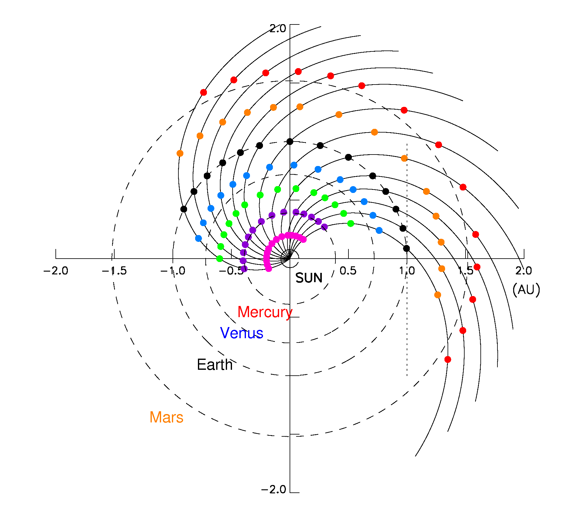
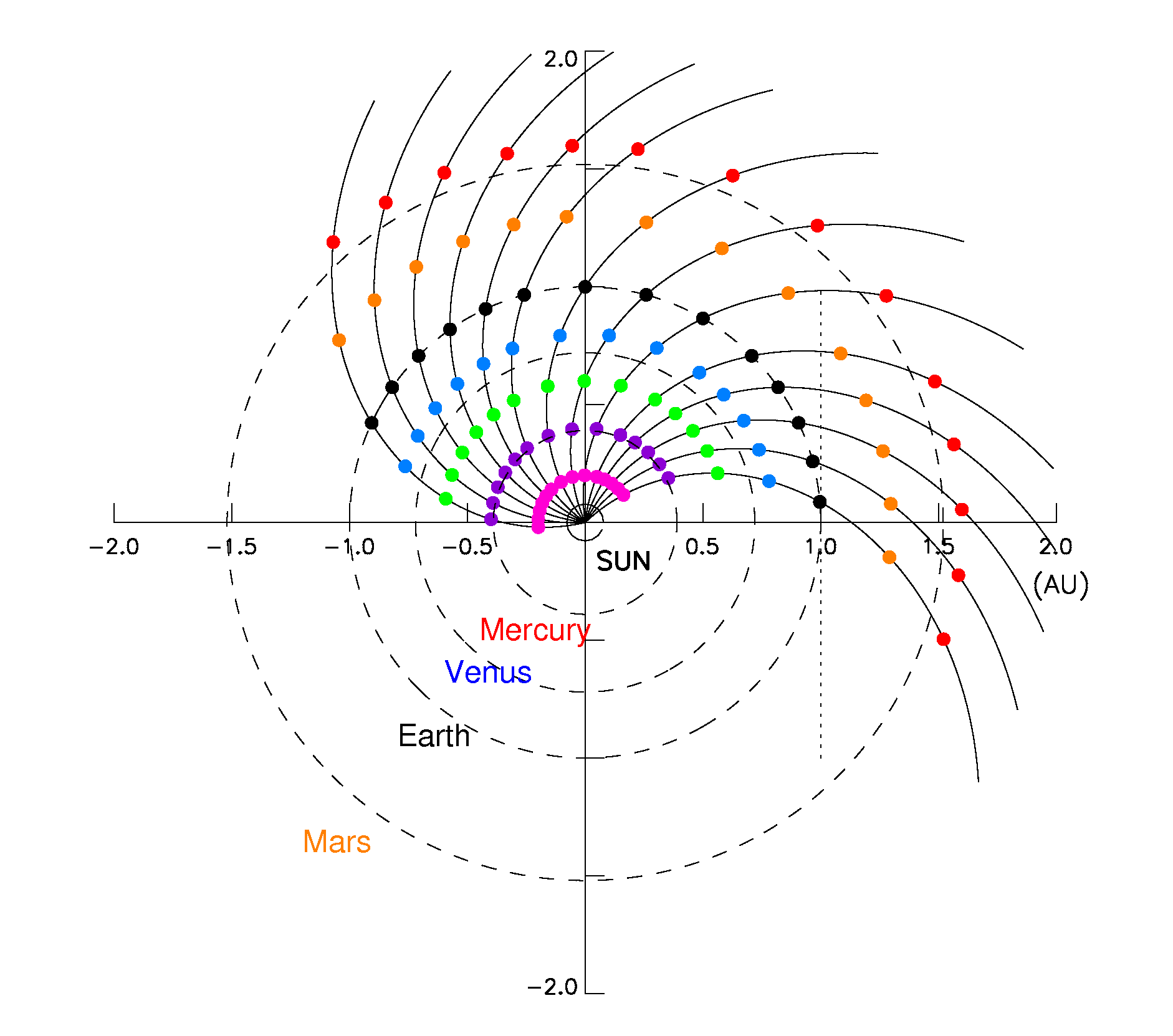
The 249 out of the 263 SEP events events observed at 1 AU between January 1988 and March 2013, contained in the SEPEM Reference Event list (REL), are classified into one of the ten event categories and the corresponding radial scales are applied. This subset of REL is hereafter named as the SEPEM Radial-dependent Reference proton Event List (SREL). In this way, the event list at 1 AU is replicated at seven heliocentric radial distances between 0.2 AU (approximately, half the mean distance of Mercury to the Sun) and 1.6 AU (Mars orbit); thus, allowing the inclusion of interplanetary missions in the SEPEM/SAT. The output of SOLPENCO2 consists of two files: one containing the scaled-to-observed (1 AU) peak intensity ratios for each of the 249 SEP events and for seven virtual observers located at 0.2, 0.4, 0.6, 0.8, 1.0, 1.3 and 1.6 AU; and the other one containing the corresponding SEP event fluence ratios. As shown in Figure 1, the virtual observers are placed along the same interplanetary magnetic field (IMF) line as the 1 AU-observer (i.e. the Earth’s nominal magnetic field line connecting with the Sun).

SOLPENCO2 is designed for the description of gradual solar proton events, originating from any heliolongitude (the range of values is shown in Figure 1) as seen from virtual observers located within 0.2 AU and 1.6 AU. For any modelled event, the tool provides the proton differential intensity-time profiles for the reference energy channels defined in SEPEM (from 5 MeV to 200 MeV, [7]) plus a higher energy channel up to 300 MeV [11].


Figure 1. Location of the observers for the slow (left) and the fast (right) wind regimes simulated.

The SEP intensity profiles depend on how the magnetic connection of the spacecraft (the observer) is established with the particle source, on how efficiently protons are accelerated and injected by the shock into the connecting magnetic flux tube(s), and on how the IMF irregularities modulate this population during its journey in space [12]. To generate the SOLPENCO2 synthetic SEP events, a new MHD model was developed for the simulation of the CME-driven shocks from near Sun to Mars orbit [8 and13]. The shock propagation model provides values of the MHD variables at the point of the shock front that magnetically connected to the observer (or cobpoint) [14 and 15]; these values are used as inputs to a particle transport model [5]. These models allow computing the injection rate of shock-accelerated particles at a given time, Q, which is a source term in the transport equation describing the propagation of protons along the IMF, towards the observer.

Figure 1 depicts the longitudinal extension covered by SOLPENCO2 for each radial position of the observer. SOLPENCO2 includes simulations of the interplanetary shock propagation on top of two different solar wind regimes, with a speed of 365 km/s, at 1 AU, for the slow case (left panel of Figure 1) and with a speed of 595 km/s for the fast case (right panel of Figure 1).

For instance, the solar source longitudinal span covered by the simulations provided in SOLPENCO2 at 1 AU extends from W85 to E65. In this range 14 different observers (or solar source sites) are considered: W85, W75, W65, W55, W45, W30, W15, W00, E15, E25, E35, E45, E55 and E65.

For each kind of solar wind regime, SOLPENCO2 includes 8 different shock simulations characterised by different times of the shock arrival to 1 AU: from 17 to 48 hours on top of the fast wind and from 24 to 67 hours on top of the slow wind. Also, to try to cover a larger number of possible scenarios than in SOLPENCO, the shock simulations are performed for two types of shocks according to their longitudinal extension: narrow and wide shocks. Hence, the shock data base contains the cobpoint for 12,544 scenarios (7 radial distances x 14 heliolongitudes x 4 particle transport conditions x 16 shocks x 2 solar winds). Hence, using this data set, it would be possible to generate large data base of synthetic SEP intensity-time profiles with SOLPENCO2.

Any other intermediate solar-interplanetary scenarios not stored in the SOLPENCO2 data base is derived by interpolation. SOLPENCO2 uses the algorithms developed in SOLPENCO to interpolate among the four pre-calculated gradual SEPs profiles which have the closest angular positions and transit times of the shock (from the Sun to the observer) to the corresponding observed values for a given event. In this way, it is possible to produce within minutes a synthetic SEP event for a given observed event at 1 AU or at non-Earth heliocentric radial distances.

The MHD simulation of interplanetary shocks

The evolution of collisionless, travelling and expanding interplanetary shocks from Sun to Mars orbit was modelled by means of a two dimensional (2D) MHD model [8]. For the background solar wind plasma a polytropic relation is assumed between density and pressure with a radial varying polytropic index [13]. A comparison of the results from this 2D MHD model with a newer one using a heating source function for the solar wind is presented and discussed in [9]. The 2D MHD model [8,13] permits the application of two different regimes: fast/low density/high temperature or slow/high density/low temperature solar wind. The MHD model assumes spherical geometry with a radial extent in the equatorial plane from 1.03 solar radii to 1.6 AU. As the shock evolves, the cobpoint slides along the shock front scanning regions of different MHD properties. Figure 2 shows a snapshot of one of these shock simulations with several IMF lines. For the synthesis of each SEP event profile, a simulation of the shock propagation was performed to compute the evolution of its strength along the shock front.

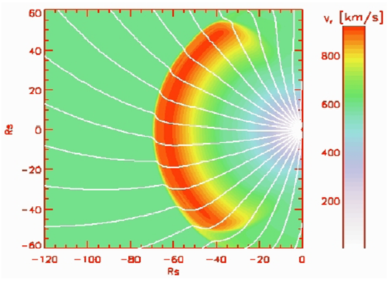Figure 2. Snapshot of an interplanetary shock simulation propagating from Sun to ~0.5 AU. Solar wind plasma speed is colour coded (as indicated) and a set of IMF lines (white lines) is also shown.

The strength of the shock is characterised by means of the different plasma values at the cobpoint [15]; namely: the normalised downstream-to-upstream plasma velocity jump, VR; the magnetic downstream to upstream ratio, BR; and the local angle between the upstream IMF and the normal to the shock front, θ_Bn [5 and 15]. As the shocks expands and evolves in space, the cobpoint slides along the front of the shock and hence, the plasma values change with time (as they depend on the local unperturbed upstream and on the shocked downstream solar wind conditions). Figure 3 (from [3]) sketches this concept: particles accelerated at the front of the shock are injected in the magnetic field lines connecting the observer (black diamond) with the shock at the cobpoint (red point); in this particular scenario, the position of the cobpoint moves towards the nose of the shock (red arrow), consequently, the efficiency of the injection of shock-accelerated particles increases. Therefore, the values at the cobpoint, for a given time and a given observer considered in the data base of SOLPENCO2 can be derived.

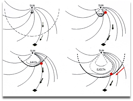Figure 3. Cartoon showing the evolution of the cobpoint with respect to the front of the CME-driven shock and the position of the observer, for a given solar-interplanetary scenario.

The particle transport equation

The model adopted in [5] for the simulation of the interplanetary propagation of protons uses the transport equation derived by [16] and [17]. The transport model requires as input the following variables, derived from the shock simulations performed with the MHD model: the position of the cobpoint as the shock progresses and expands from near Sun, the transit speed of the shock and the values of VR, at the cobpoint. The basic parameters of the transport model, as used here, are the mean free path of the protons, λ, the injection rate of shock-accelerated protons in interplanetary space, Q (phase space density) and the dependence with the energy of this injection rate (characterized by a spectral index, γ).

This injection rate changes with time, as it depends on the existing shock jump conditions at the cobpoint. Q is the source term in the transport equation: it gives the efficiency of the shock as injector of accelerated particles in interplanetary medium. The mean free path, λ, describes the propagation of particles in the diffusive-focused transport model which is the result of the interaction between energetic particles and IMF irregularities in the quasi-linear approximation [18]. For the description of some events, the presence of a turbulent magnetic foreshock region is required to reproduce the flux and the anisotropy values observed in the spiky energetic storm particle (ESP) component at the shock arrival. This foreshock is represented by a region of a given width just ahead of the shock, whose particle mean free path is much smaller than that in the rest of the upstream medium [5]. The transport equation is solved for each shock scenario by using a numerical algorithm that assumes that the inner boundary limit is at the radial distance of the cobpoint, which evolves as the shock propagates [5].

Deriving the injection rate and its energy dependence

Up to now, the precise details on how the 'acceleration efficiency' of the evolving shock behaves are neither completely clear nor quantified yet. A conceptual point of the shock-and-particle model in which SOLPENCO2 tool relies is the connection of the evolving MHD variables at the cobpoint with the injection rate of shock-accelerated particles; in other words, the Q(VR)-relation derived by Lario et al [5], already applied in different situations (i.e., Aran et al. [19] and [3]). This relation implies to assume a functional dependence between Q and VR variables at the cobpoint:

(1)

where k is a proportionality factor. This expression allows the modeller to relate the dynamic evolution of the shock strength at the cobpoint to the rate at which shock-accelerated particles are injected into the interplanetary medium. For a given SEP event, the flux and anisotropy profiles are fitted for one energy channel E₀. This yields λ₀ and Q₀, as well as their evolution in the upstream region of the event. The dependence of Q(E) and λ(E) on the energy E is then derived by obtaining the best possible eyeball simultaneous fit to a large number of observed flux profiles (more than twenty) at selected energies, plus the simultaneous fit to the corresponding first order anisotropy profiles when available [3, 4, 8, 9, 19].

To model the reference events with SOLPENCO2, averaged values for k and Q₀ are assumed. Then, the variation of the injection rate for each scenario is computed by using Eq. (1) because the values of VR are derived from the MHD simulation of the corresponding shock.

The main difference between SOLPENCO and SOLPENCO2 lies in the purpose of the two tools. SOLPENCO is a stand-alone tool ready to be operated by any user with some knowledge of SEP events, while SOLPENCO2 is designed for providing inputs to the SEPEM interplanetary statistical analysis model. SOLPENCO2 uses scaling factors that are specific for the reference events, in order to match 1 AU data, whereas SOLPENCO used a universal scaling factor for its SEP events database. Both, however, share the same modular approach, which would enable the possibility of developing another tool more similar to the first SOLPENCO, using the simulations available in SOLPENCO2.

SOLPENCO2 in SEPEM — Towards a statistical model away from 1 AU

SOLPENCO2 is designed for providing inputs to the SEPEM Interplanetary SEP statistical model. Isolated SEP events at 1 AU have been identified in order to calibrate the synthetic flux profiles and to determine the contribution of the downstream region to the fluence of a given event. This has required identifying the solar origin for each event of SREL, as well as the time of shock arrival and the event duration. It has been also necessary to evaluate how to reproduce compound events as defined in the statistical Analysis Tool. Finally, we produce the synthetic flux profiles at other locations than 1 AU by assuming that the observers are at the same IMF line as the observer at 1 AU (i.e., the Earth). This allows calculating the peak intensity and fluence values for different energies and at other six radial distances, from 0.2 AU to 1.6 AU. Figure 4 shows an example of the peak flux (dots, left vertical axis) and fluence (squares, right vertical axis) values derived, for two energies: 8.7 MeV (red) and 26.3 MeV (black).

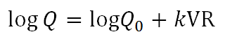
Figure 4. Example of the radial dependences for the peak flux and fluence derived for a specific solar-interplanetary scenario, for two energies.

As can be seen in Figure 4 and Figure 8 (below), the derived peak flux and fluence dependences with radial distance are different event to event and depending on the proton energy considered. The radial power-law indices derived differ from the inverse quadratic/cubic law frequently assumed and close to those derived observationally for similar scenarios [20].

The above mentioned physics-based model [8 and 9] was used to derive the radial variation of the peak intensity and fluence for ten SEP event case studies. The SEPEM statistical model is based on 1 AU cleaned data from 1973 to 2016. The solar origin of 249 out of 263 SEP events (compound and isolated) of the SREL (between January 1988 and April 2013) was determined. The intensity and maximum energy attained in the events were also analysed. Then, the SREL events were classified into the ten sub-types in order to assign to them the corresponding radial dependences. This allows to scale peak intensities and fluences to other radial distances and make use of the SEPEM statistical modelling machinery available at 1 AU [7 and 10].

Case studies: Comparing SOLPENCO2 synthetic SEP events with 1 AU data from the SREL list and the derived heliocentric radial dependences

Ten SEP events were selected from the SREL list to be reproduced with SOLPENCO2. These events are:

the 14 December 2006 SEP event,
the 10 June 2000 SEP event,
the 4 April 2000 SEP event,
the 6 June 2000 SEP event,
the 6 March 1989 SEP event,
the 13 March 2012 SEP event,
the 29 March 2001 SEP event,
the 24 September 2001 SEP event,
the 29 October 2003 SEP event,
and the 13 December 2006 SEP event.

Note that in this section, we refer to an "SEP event" following the scientific definition: a particle enhancement generated by a specific solar activity (either flare or/and CME) and often associated with interplanetary shocks. In the statistical analysis, (both at 1 AU and away from 1 AU), a particle intensity enhancement above a prescribed threshold in the 7.23—10.46 MeV channel is defined as an SEP event. Consequently, an event defined in this latter manner may be compound of different SEP events as per the former definition. In the following, when we refer to compound events, these are particle enhancements consisting of a series of SEP events defined by their solar and interplanetary (if identified) sources.

Comparison with 1 AU data

Two sets of scaling factors were established per event at 1 AU: for peak fluxes and for upstream fluences, between the observed and synthetic values. Consistency between the total fluence simulated at 1 AU and the observed value was checked by calculating the total-to-upstream observed fluence ratios.

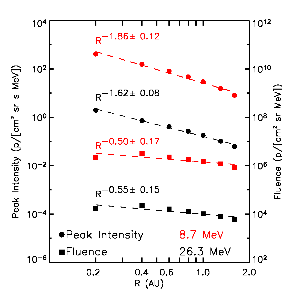
Figures 5, 6 and 7 show the comparison of the observed intensity-time profiles for the SEPEM standard differential channels and the synthetic profiles produced by SOLPENCO2 for each SEP event.

December 14, 2006 SEP event: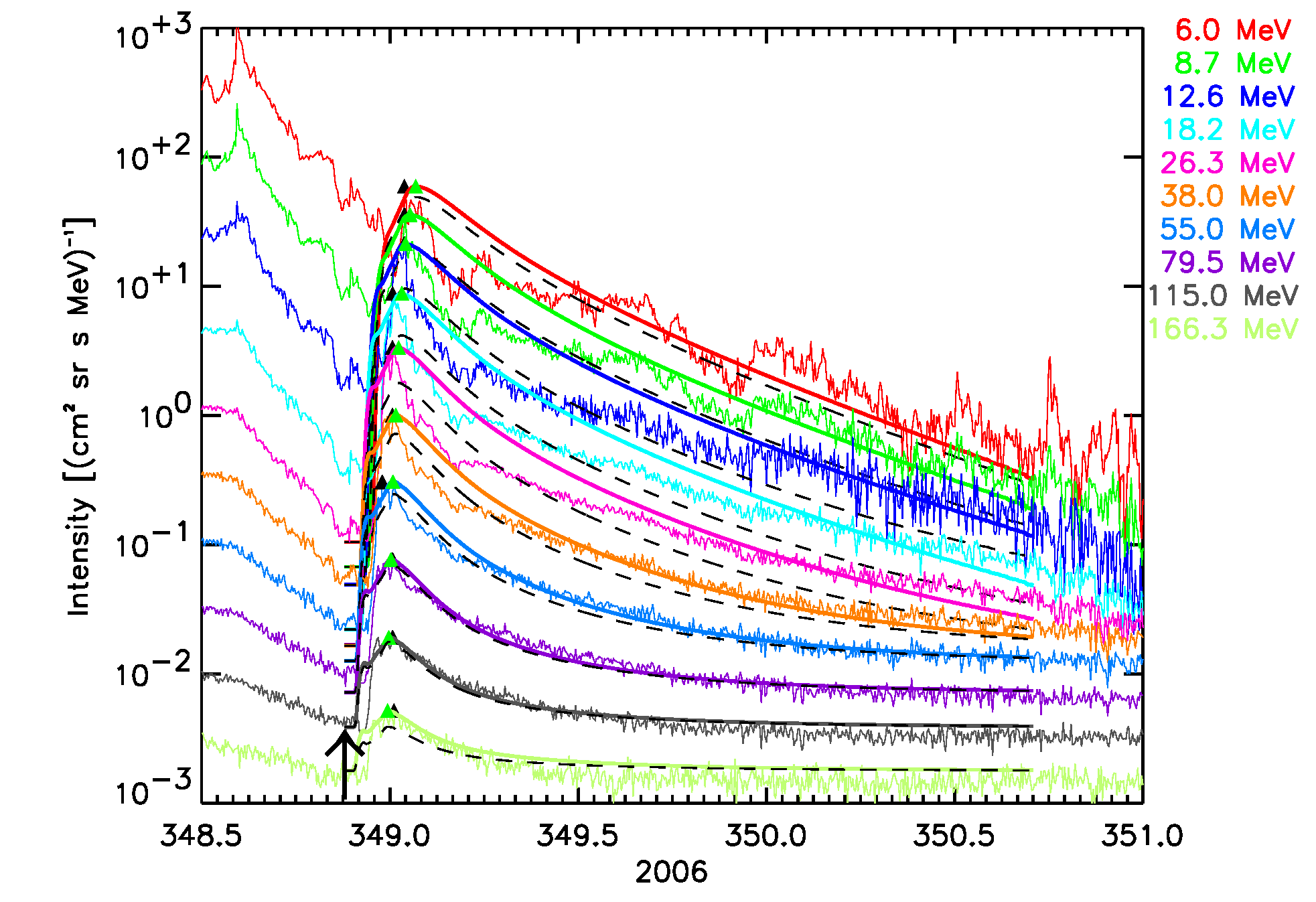
Fast wind, No shock, W44

June 10, 2000 SEP event:
Fast wind, No shock, W38

April 4, 2000 SEP event: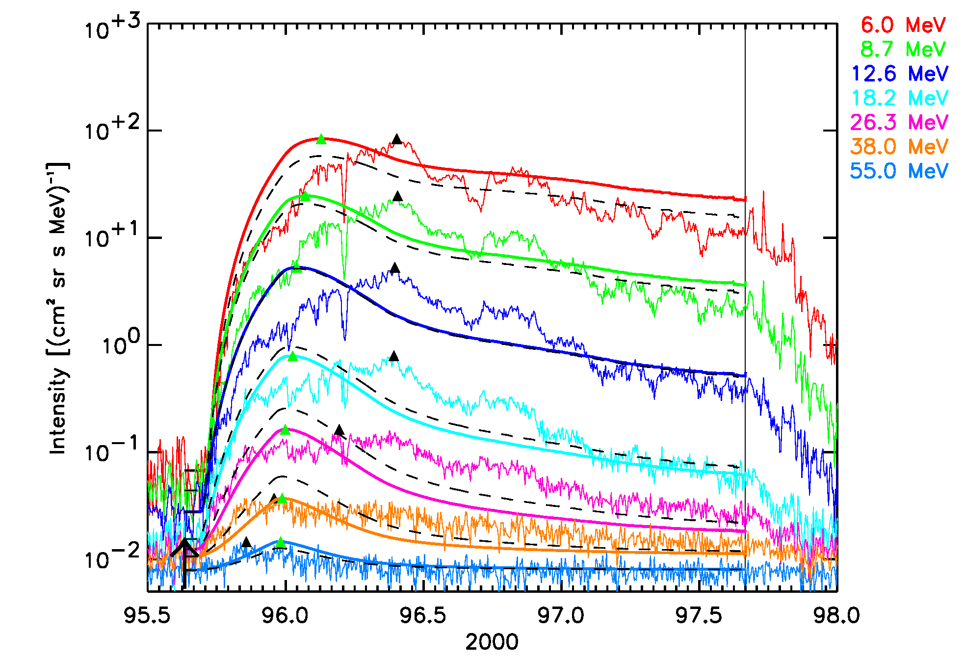
Slow wind, E < 66 MeV, W66

June 6, 2000 SEP event: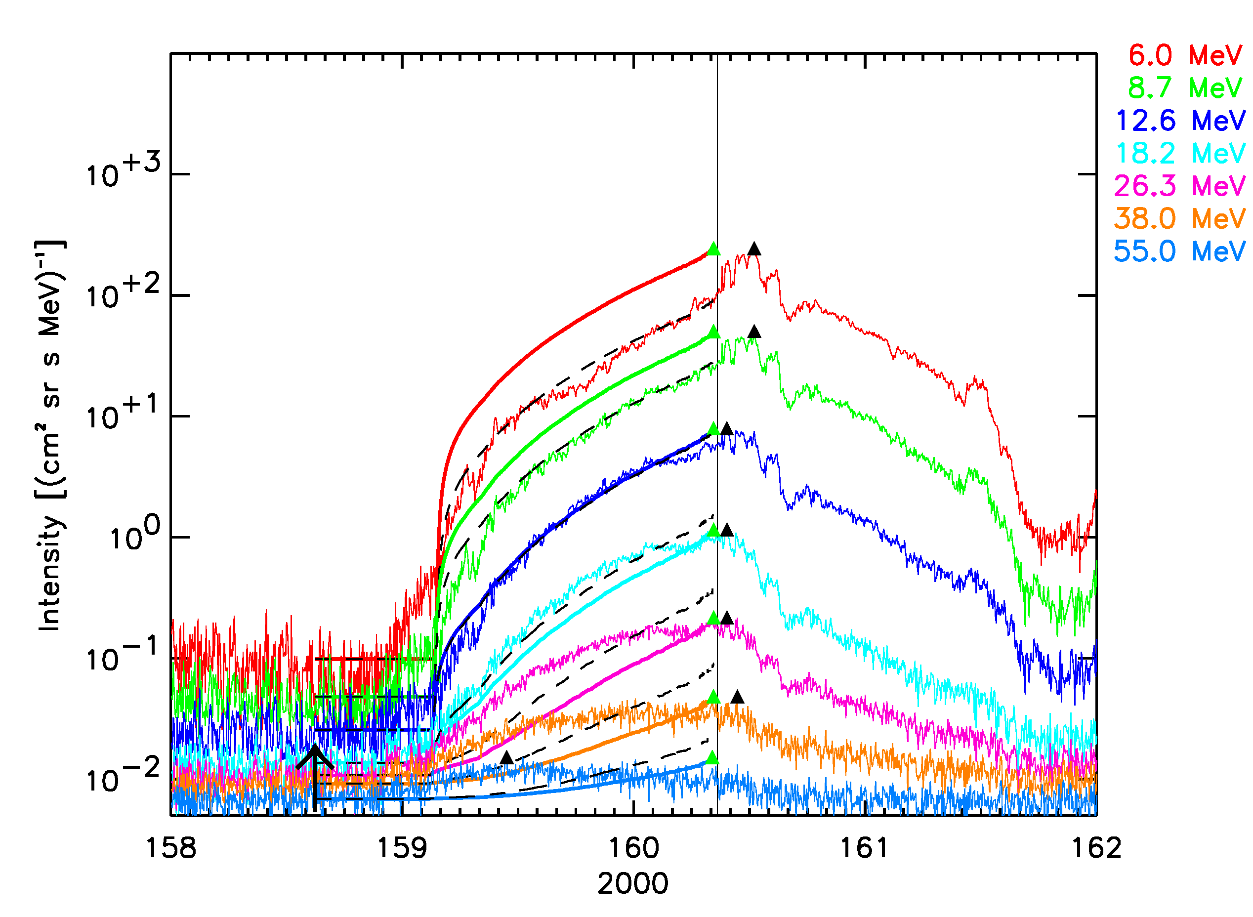
Fast wind, E < 66 MeV, E18

March 29, 2001 SEP event: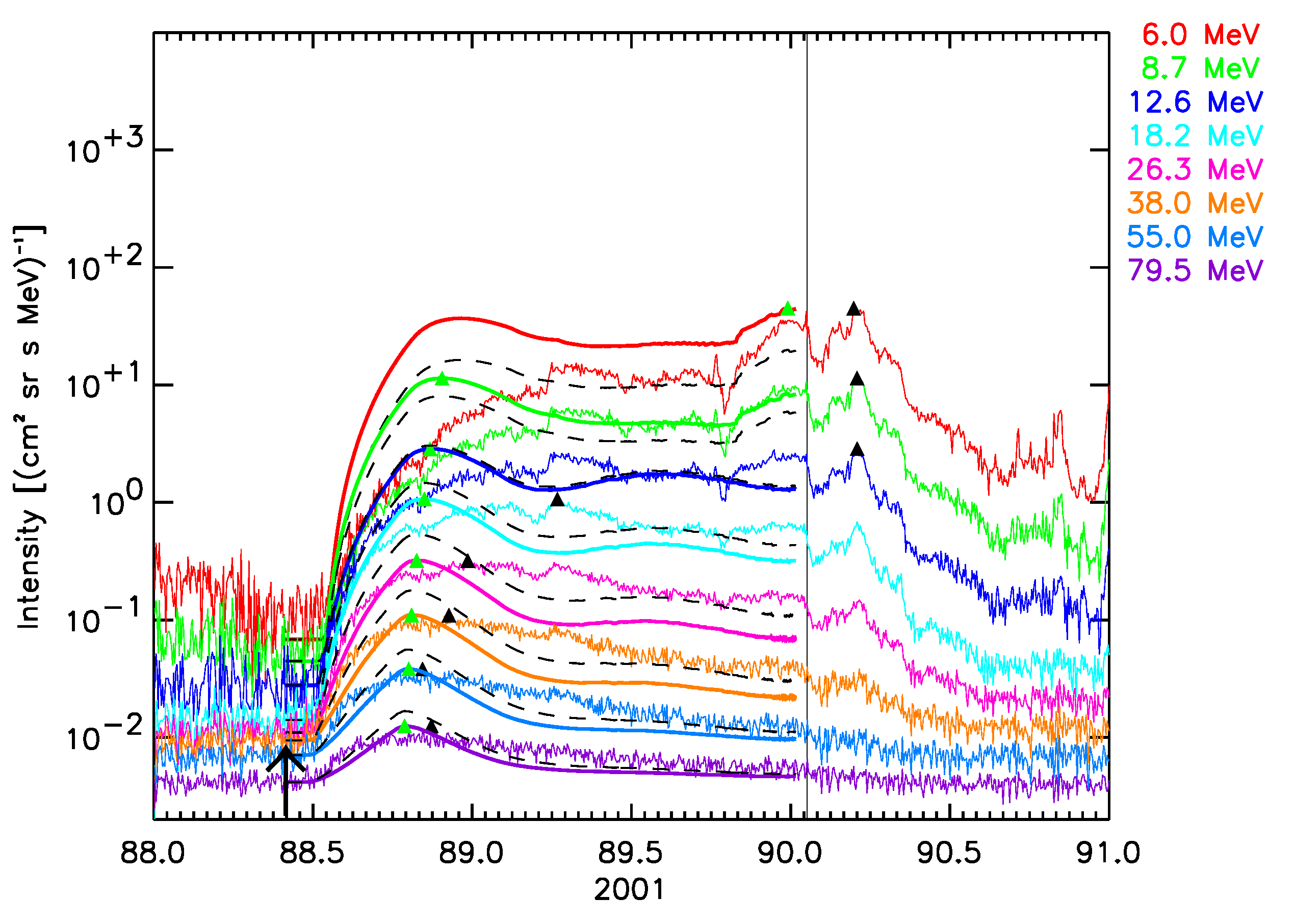
Slow wind, E > 66 MeV, W15

December 13, 2006 SEP event: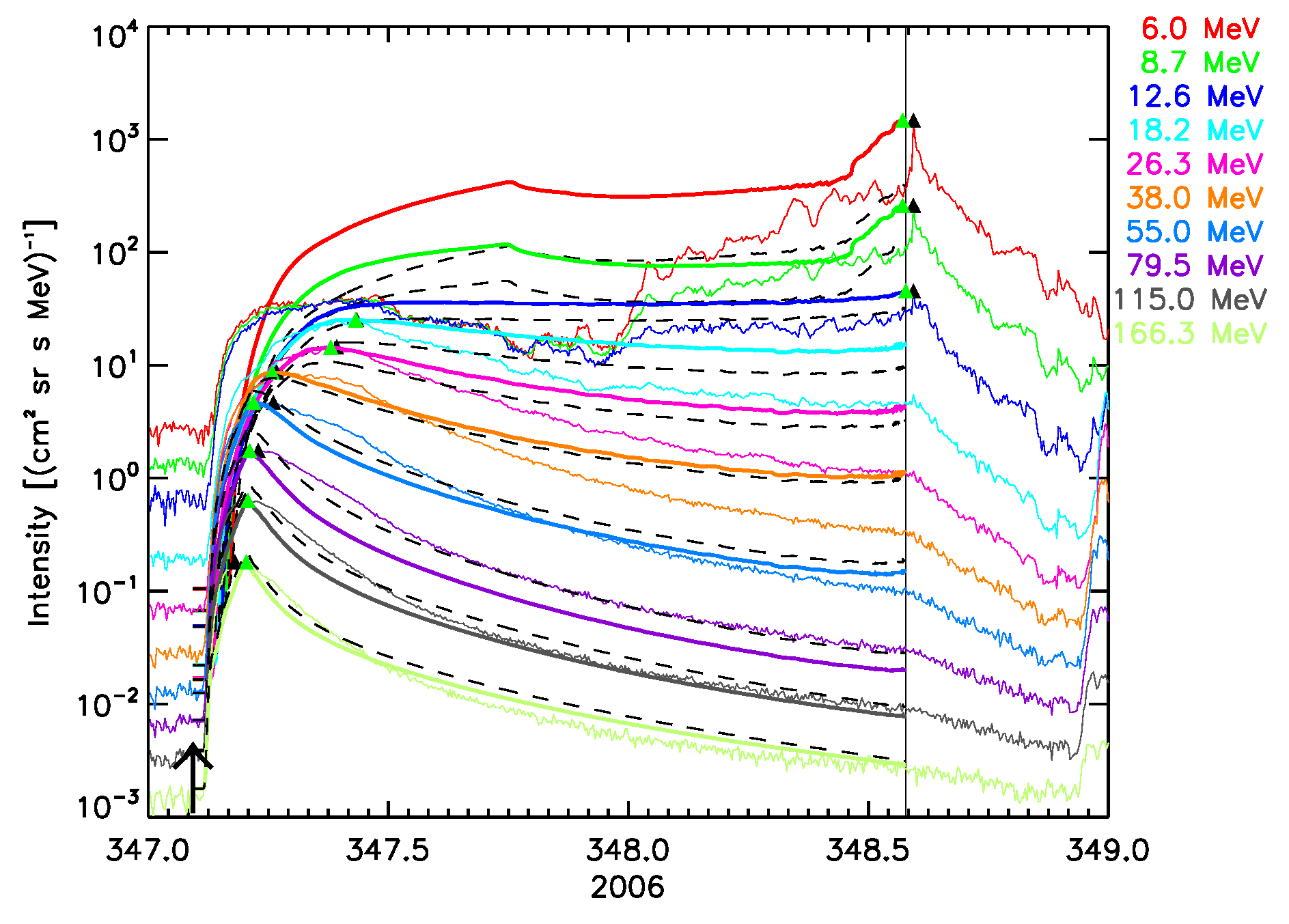
Fast wind, E > 66 MeV, W23

Figure 5. The six SEPEM reference cases, comparison with 1 AU Reference data. SOLPENCO2 synthetic flux profiles scaled per channel using: peak intensity (solid lines); upstream fluence (dashed lines). Observed and synthetic intensities are displayed for the mean energy, indicated at the right hand side of each panel (in MeV), of the SEPEM Reference Data energy channels. Peak intensities: observed (black triangles), simulated (green triangles). Vertical lines mark the passage of an interplanetary shock by the ACE spacecraft at L1.

Figure 6. Two new reference cases modelled with SOLPENCO2 (as part of SOL2UP). The synthetic flux profiles scaled per channel are shown as in Figure 5 but in this case, profiles matching the observed peak intensities are marked by dashed lines and profiles matching the upstream fluence by solid lines.

March 6, 1989 SEP event: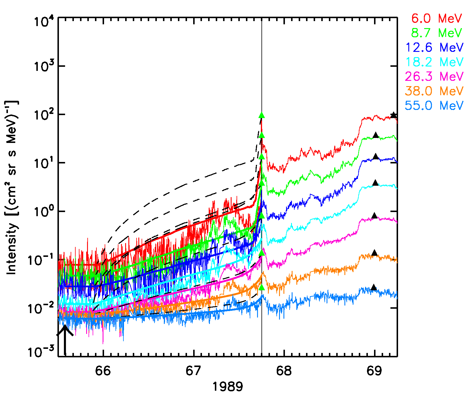
Slow wind, E < 66 MeV, E69

September 24, 2001 SEP event: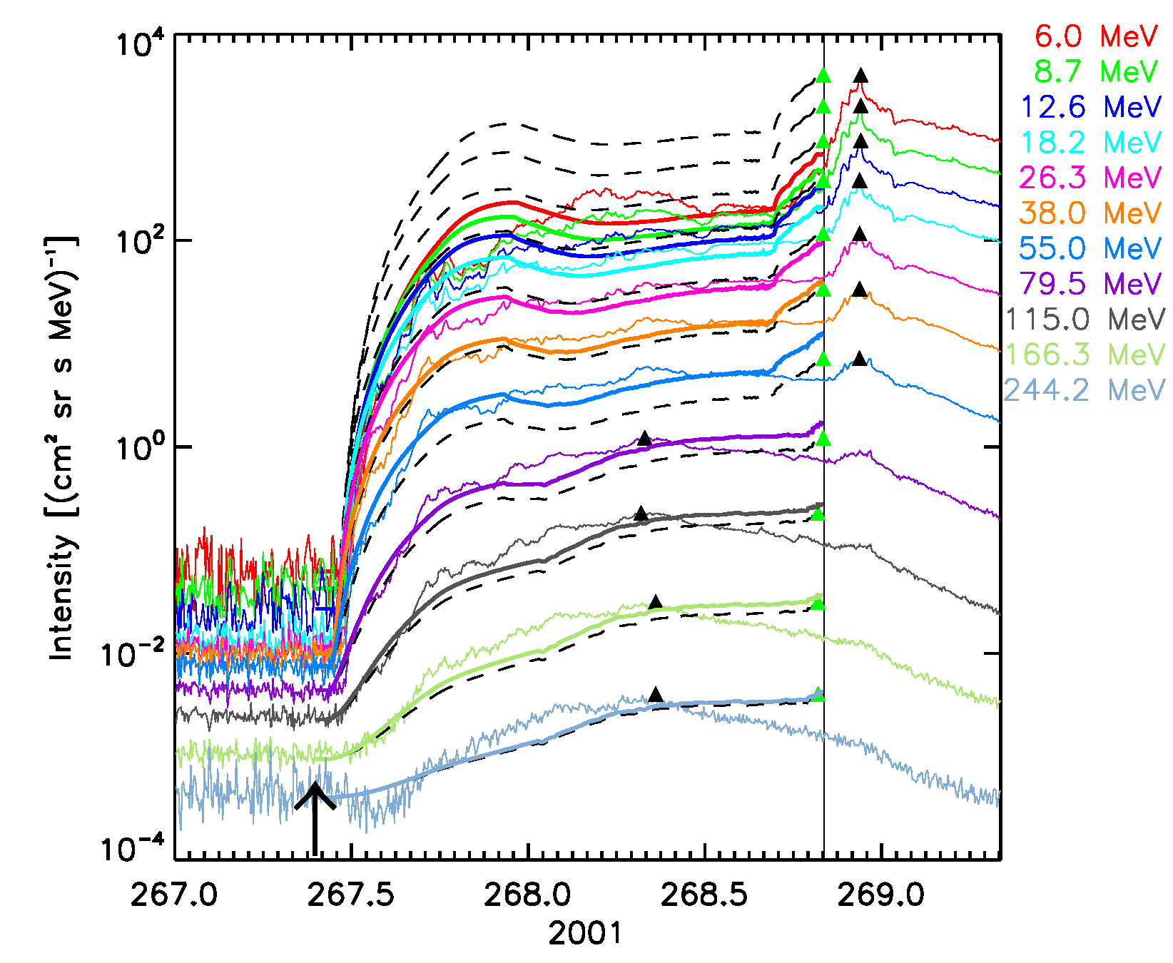
Slow wind, E > 66 MeV, E23

Figure 7. Two new reference cases modelled with SOLPENCO2 (as part of SOL2UP). The synthetic flux profiles scaled per channel are shown as in Figure 5.

March 13, 2012 SEP event: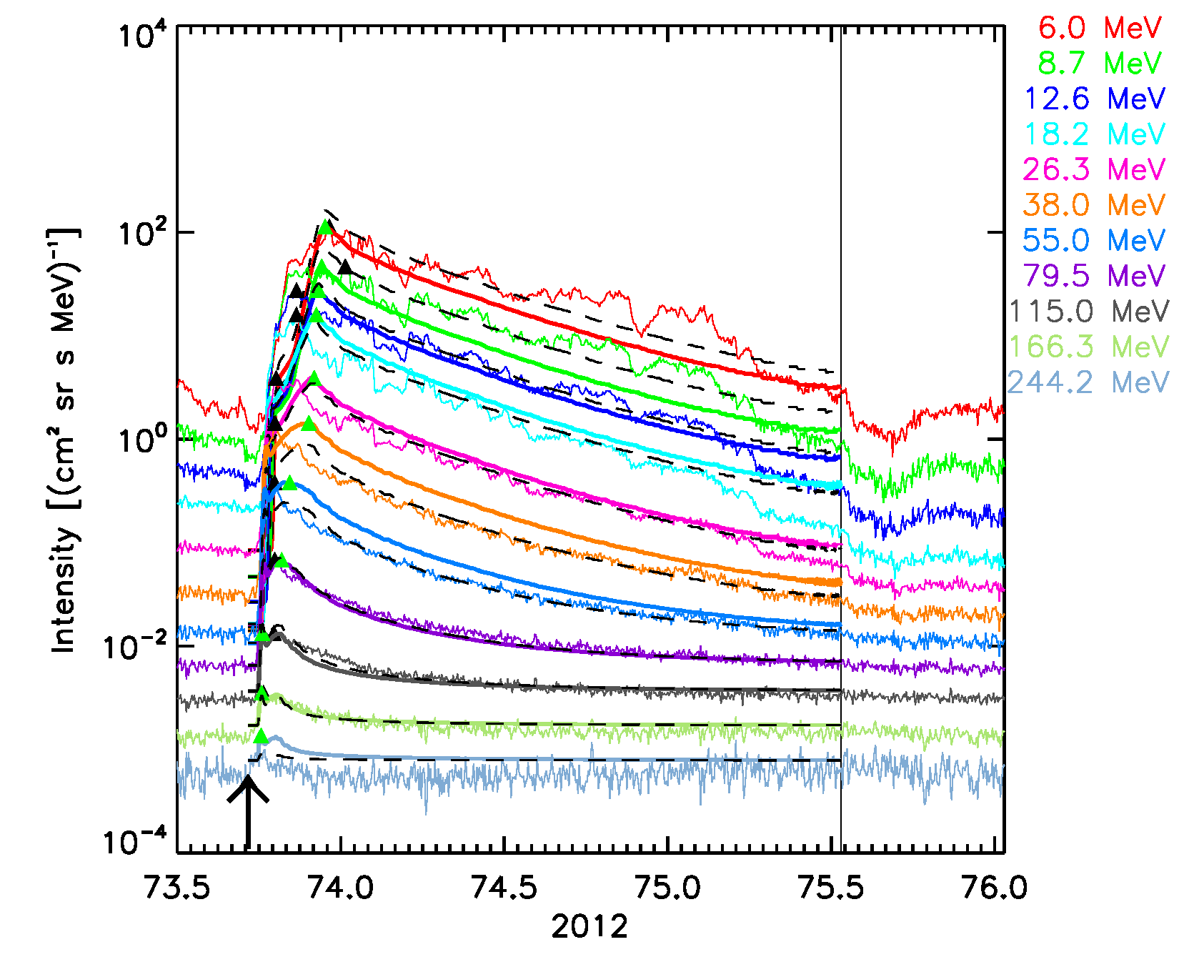
Fast wind, E < 66 MeV, E18

October 29, 2003 SEP event: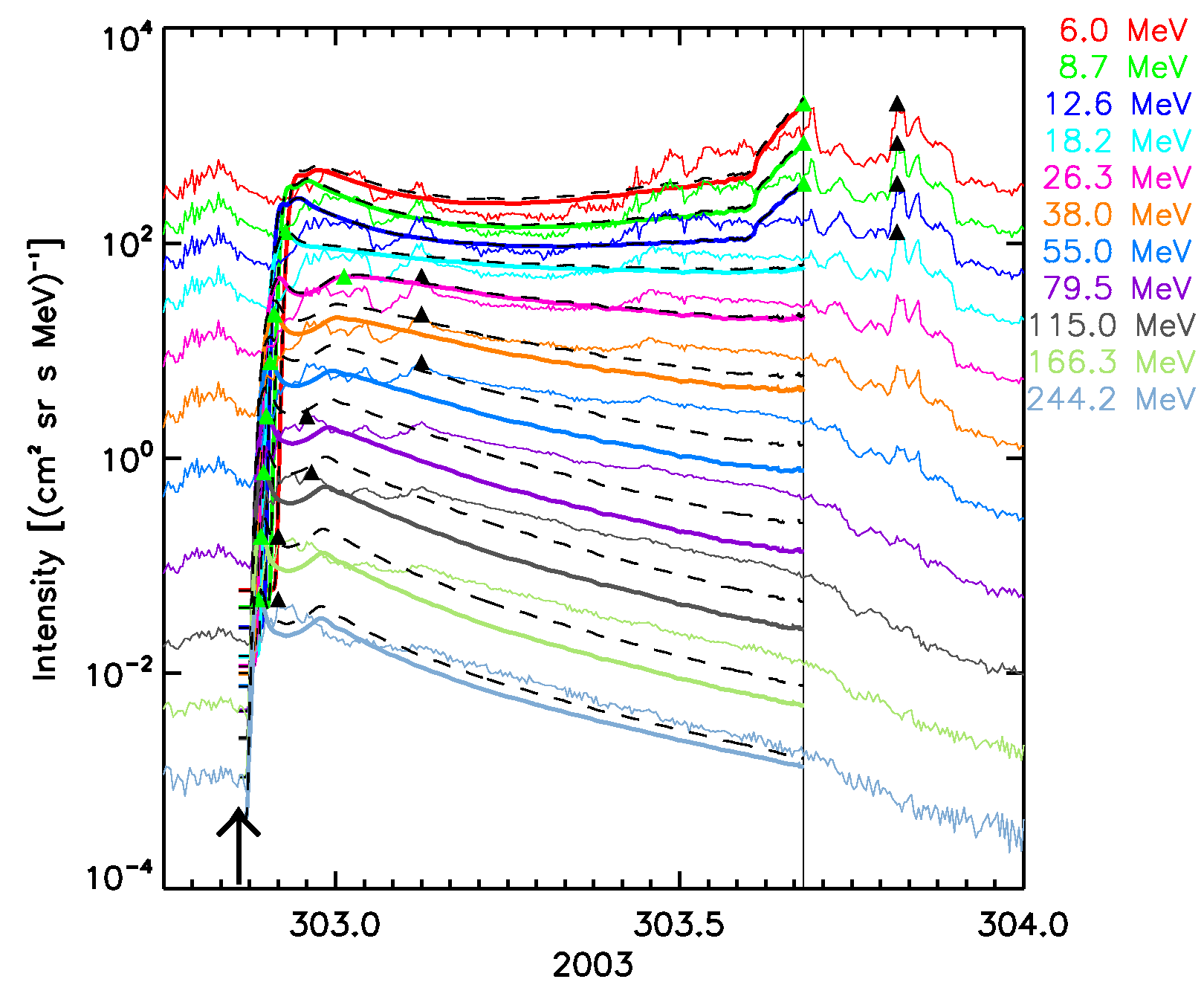
Fast wind, E > 66 MeV, W02

Upstream radial dependencies

For each simulated energy, the synthetic upstream flux profiles generated at 0.2, 0.4, 0.6, 0.8, 1.3 and 1.6 AU are scaled using these two sets of scaling factors. Note that the virtual observers are placed along the same interplanetary magnetic field line as the observer at 1 AU.

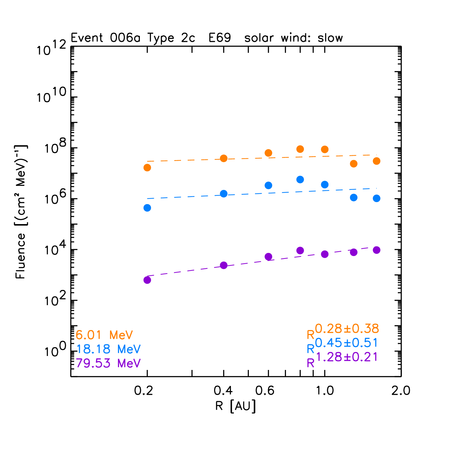
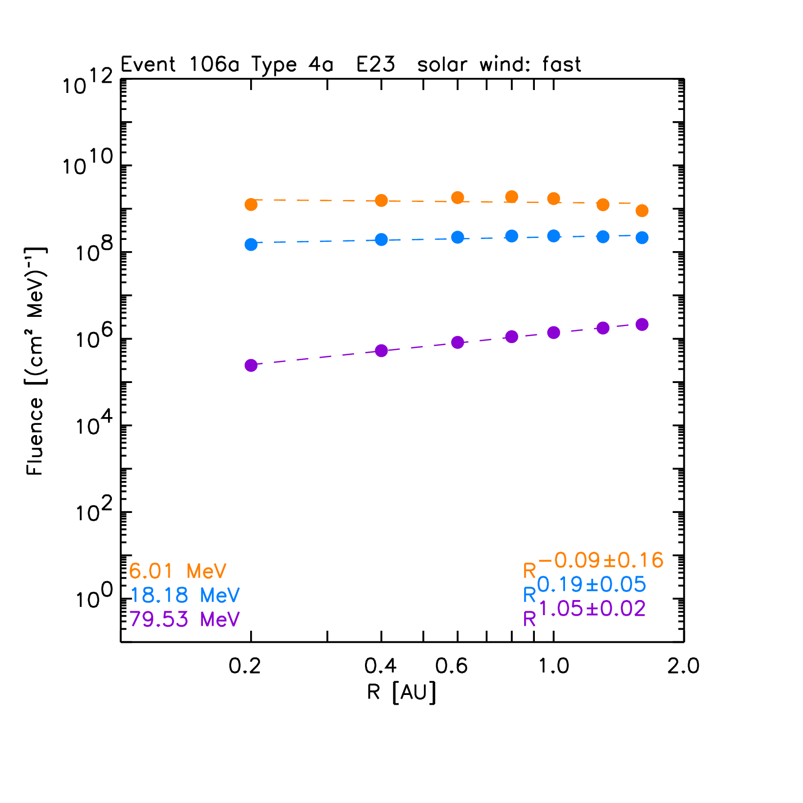
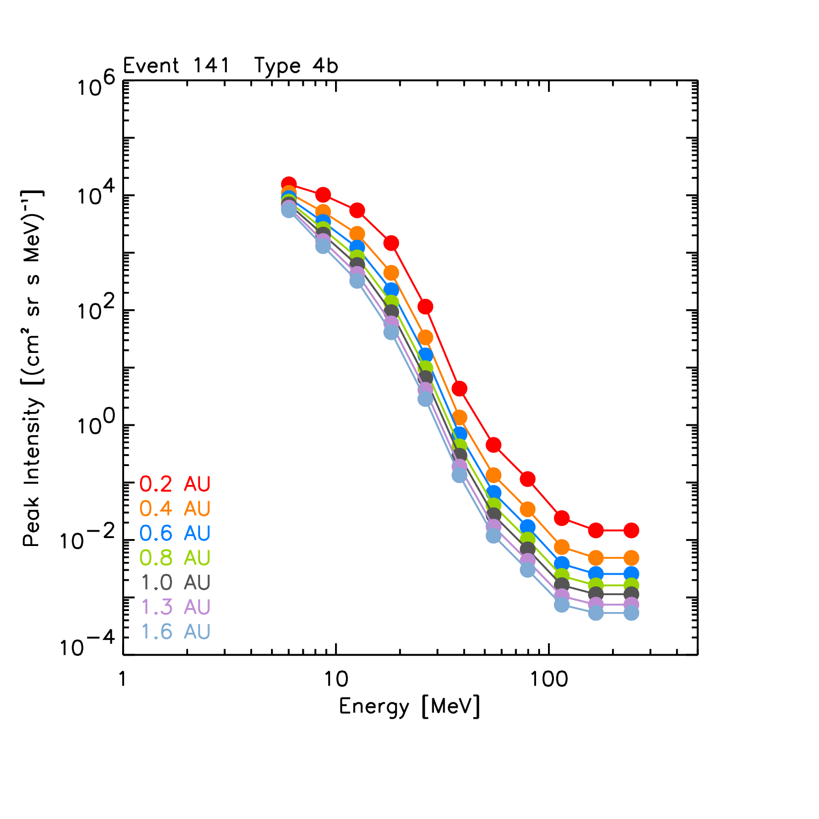
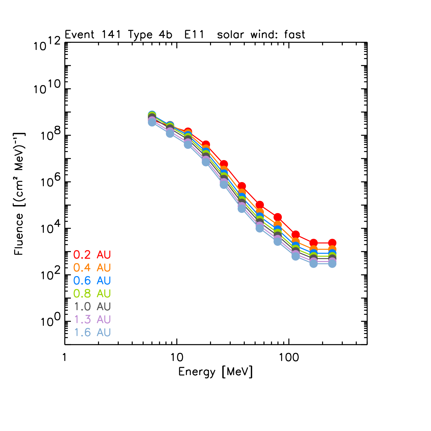
The left panels of Figure 8 show the synthetic intensity-time profiles seen by the virtual observers, for selected proton energies (indicated in each panel) for the ten reference events. The right panels of Figure 8 show the corresponding radial variations for the peak intensity (circles) and fluences (squares). A power law fit of these quantities with the radial distance (dashed lines) and the derived radial index are indicated. Note that the radial variations found for peak intensity and fluence are independent of the scaling factors but a direct result of the physical model.

At this stage, for the calculation of the total fluence of the events (indicated by squares in the right panels of the graphs in Figure 8), we assume that the observed downstream-to-total fluence ratios (DTFRs) keep constant with the radial distance. The final adopted values for the DTFRs are described below.

December 14, 2006 SEP event: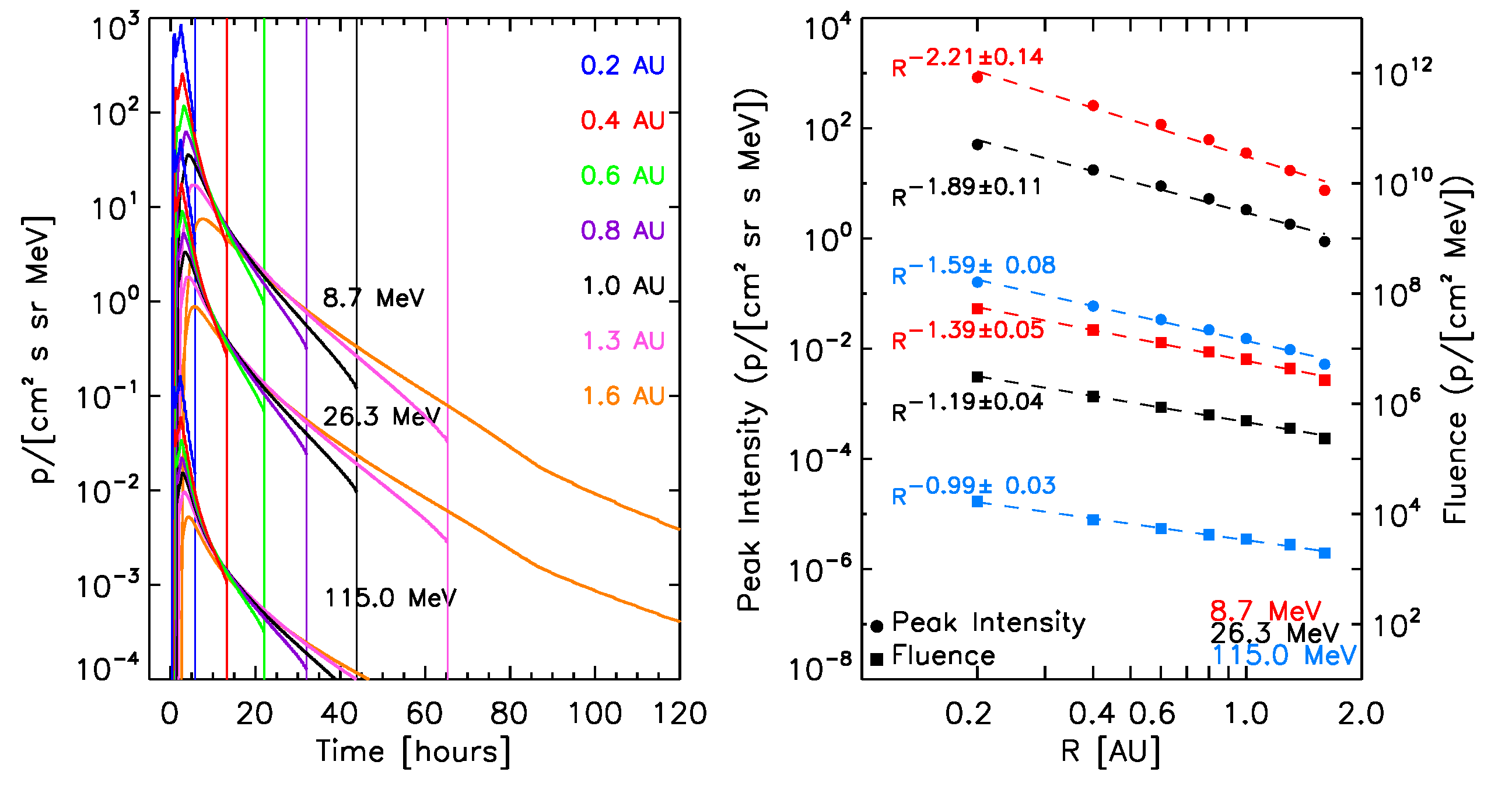

June 10, 2000 SEP event: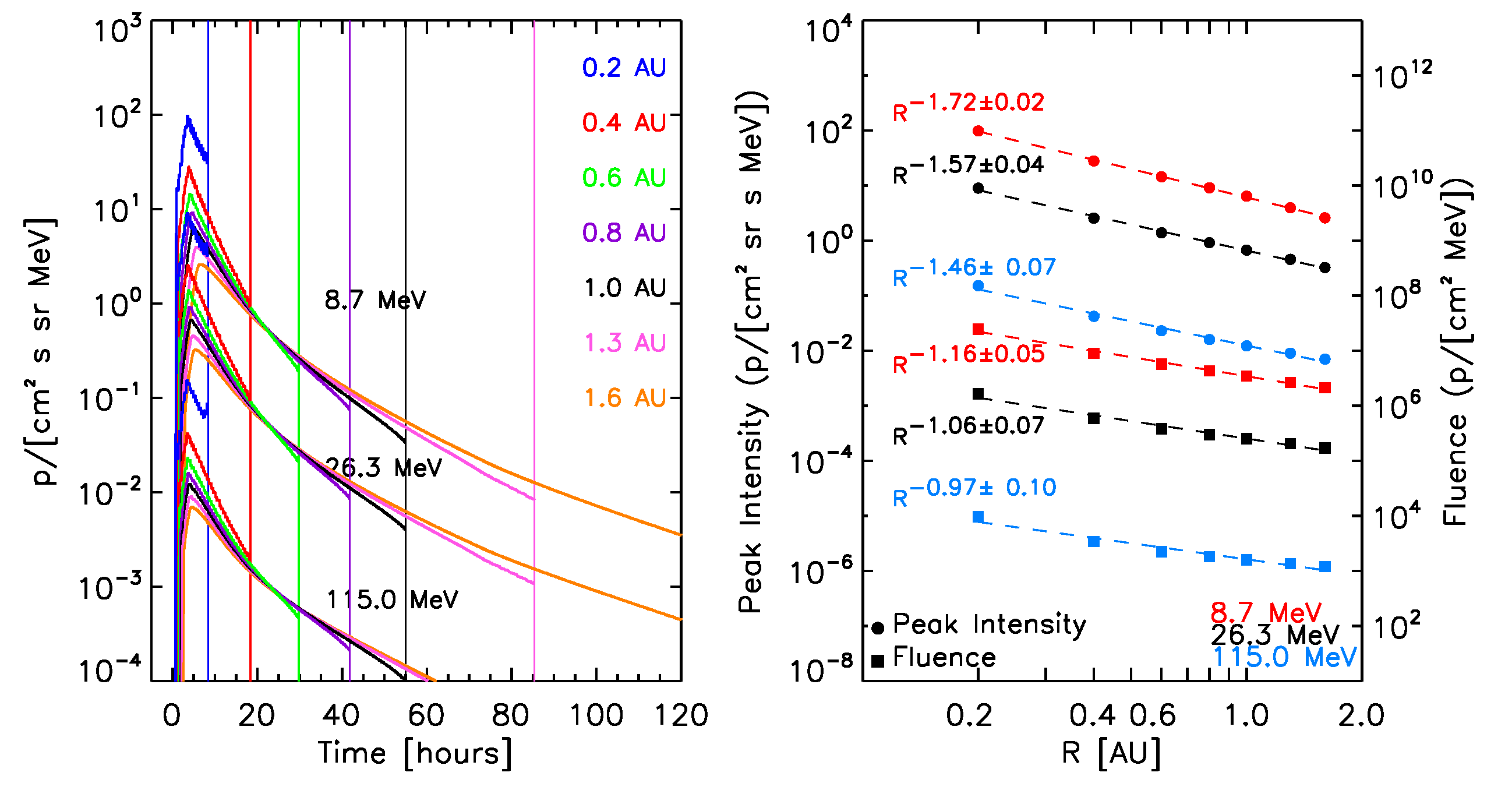

April 4, 2000 SEP event: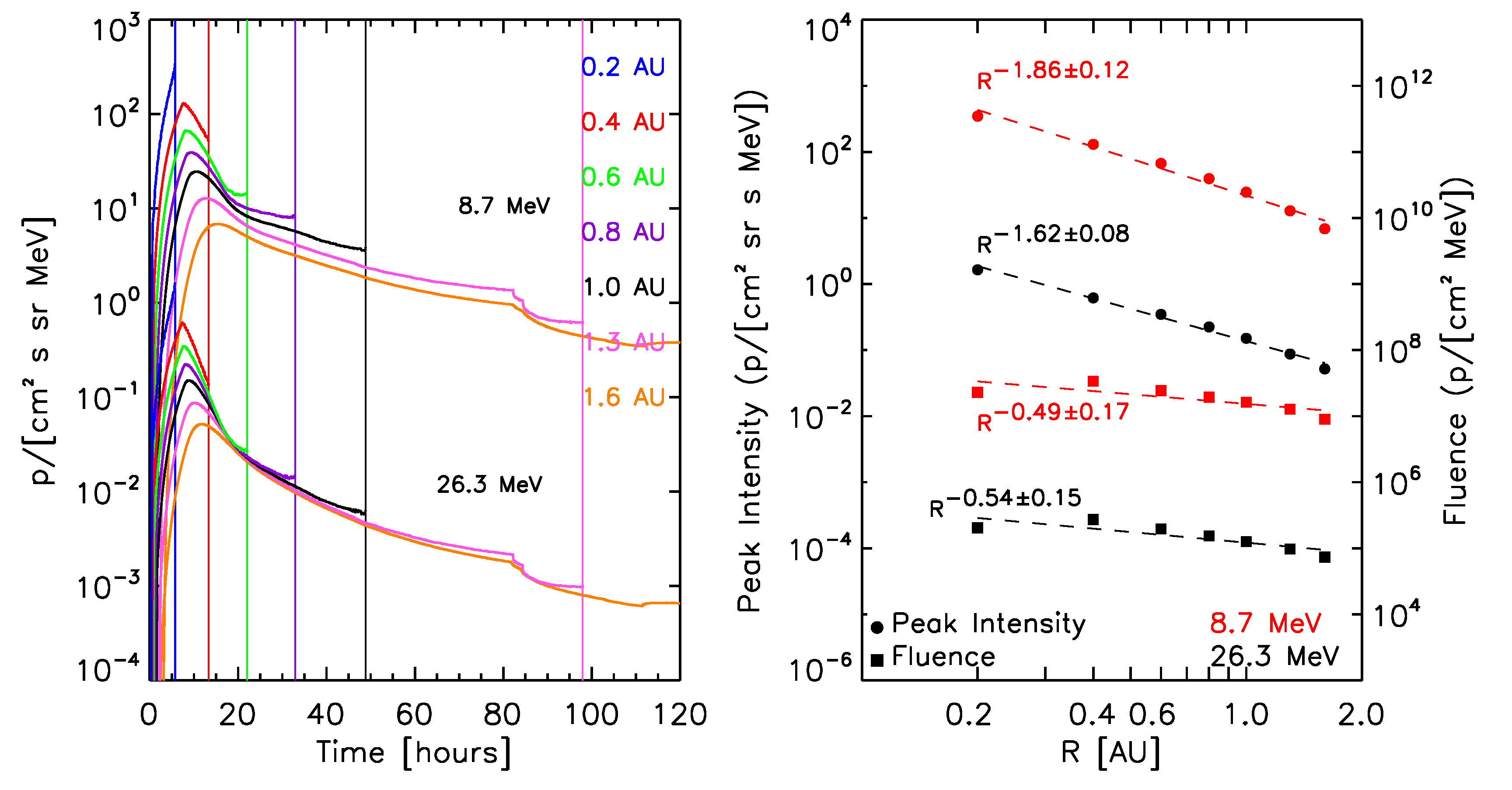

June 6, 2000 SEP event: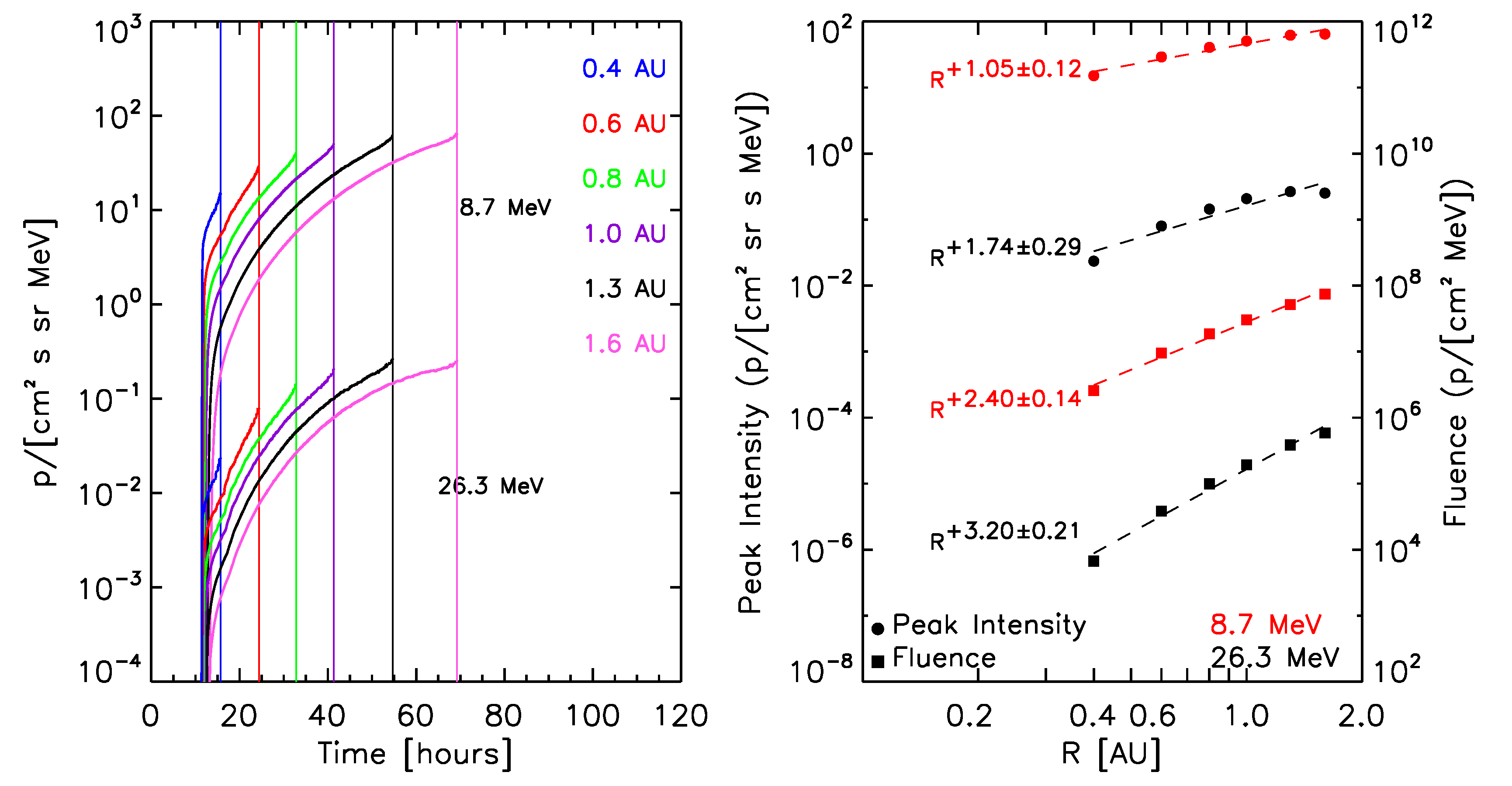

March 6, 1989 SEP event: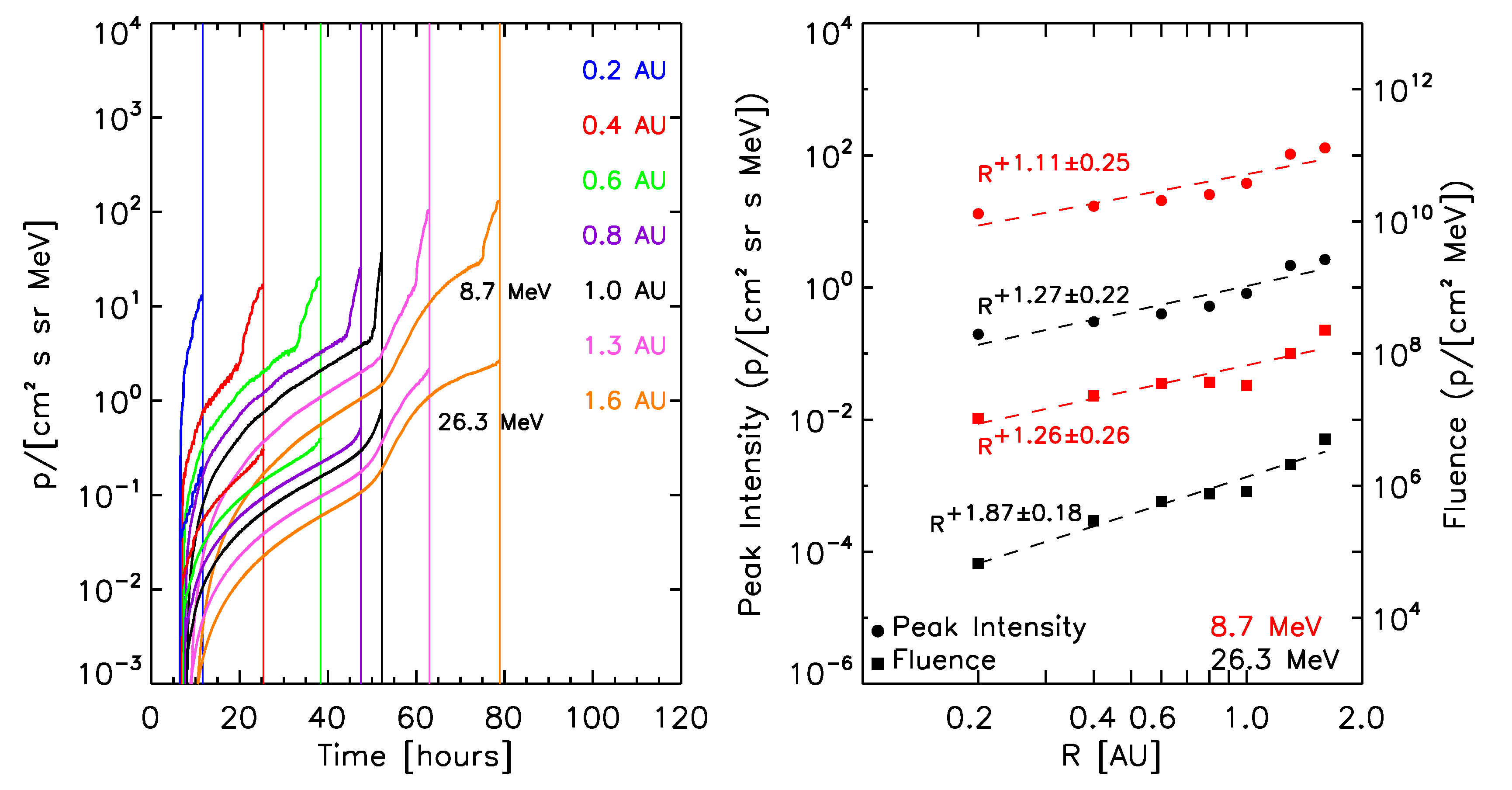

March 13, 2012 SEP event: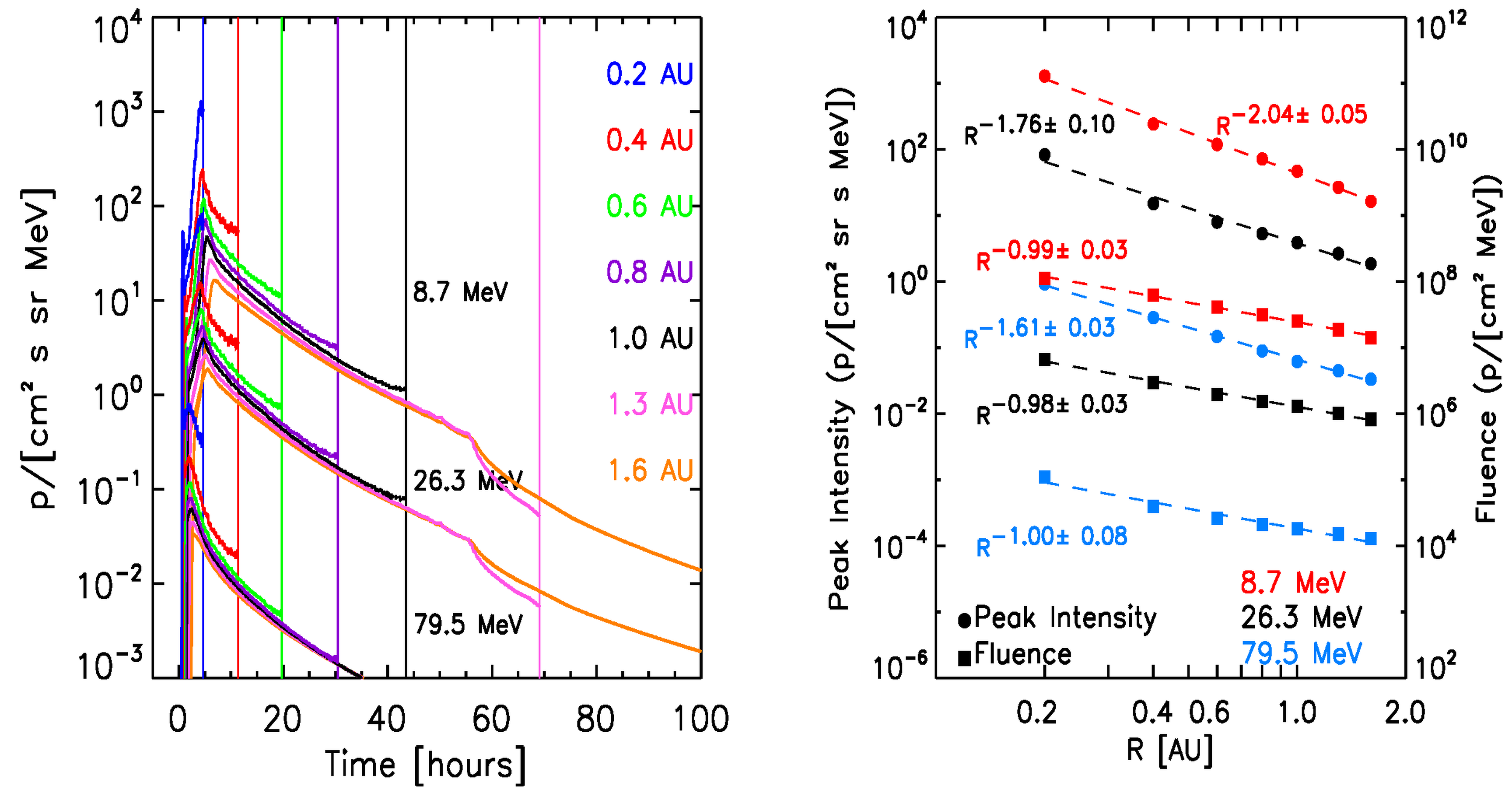

March 29, 2001 SEP event: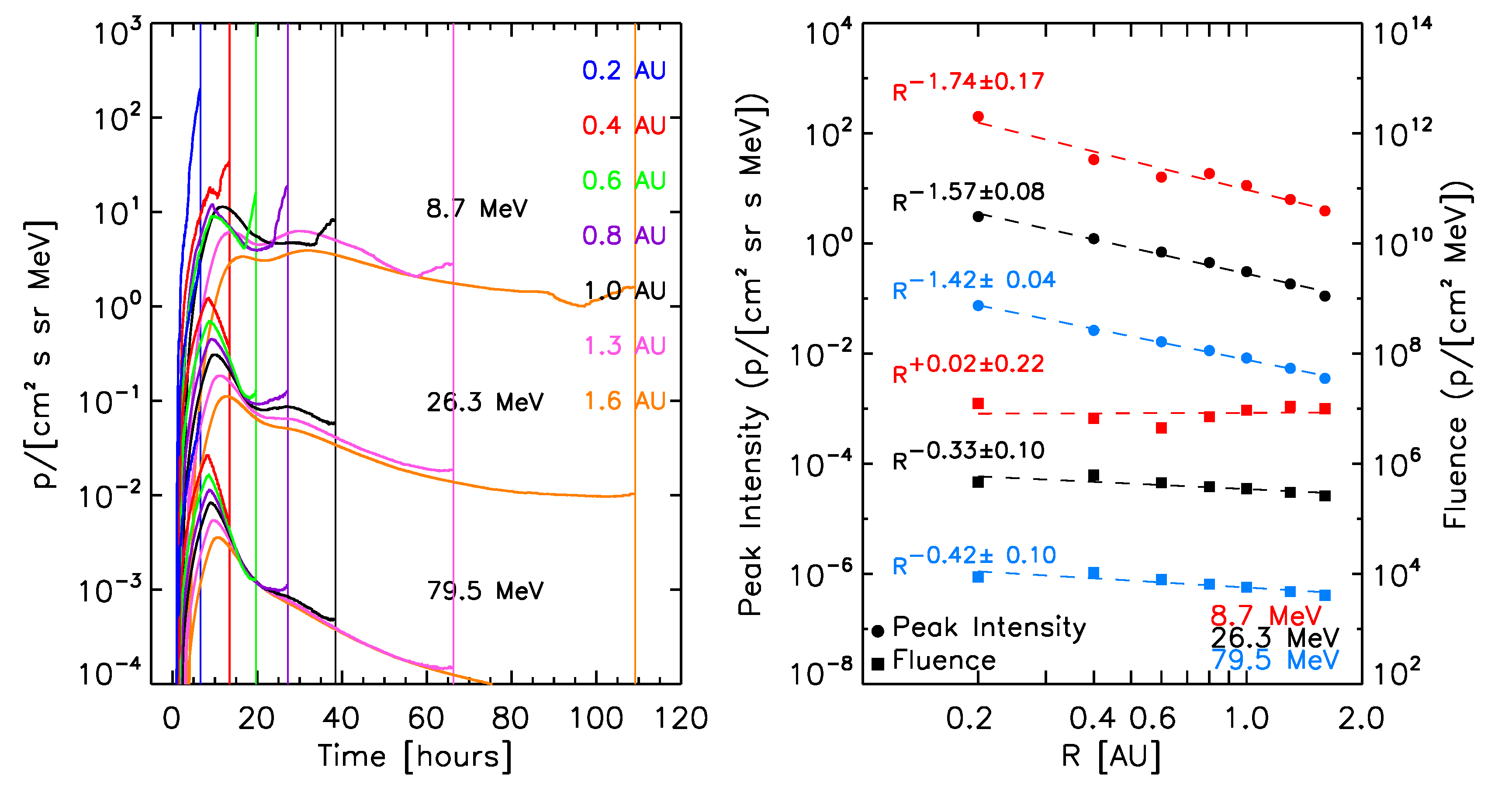

September 24, 2001 SEP event: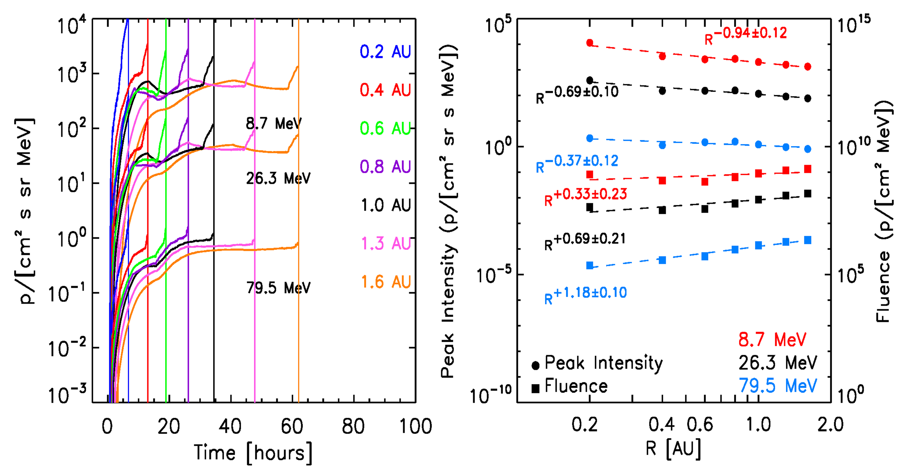

October 29, 2003 SEP event: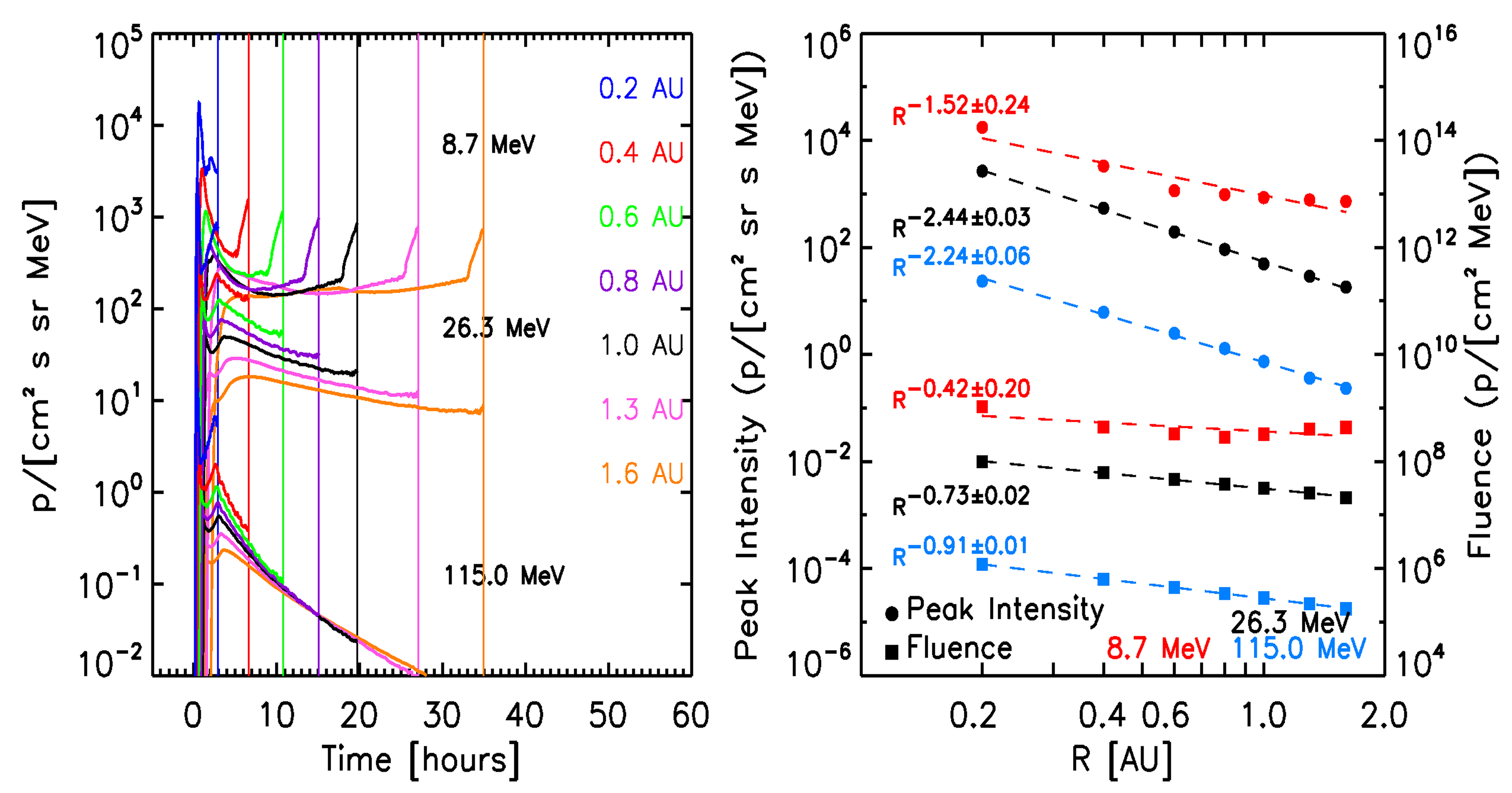

December 13, 2006 SEP event: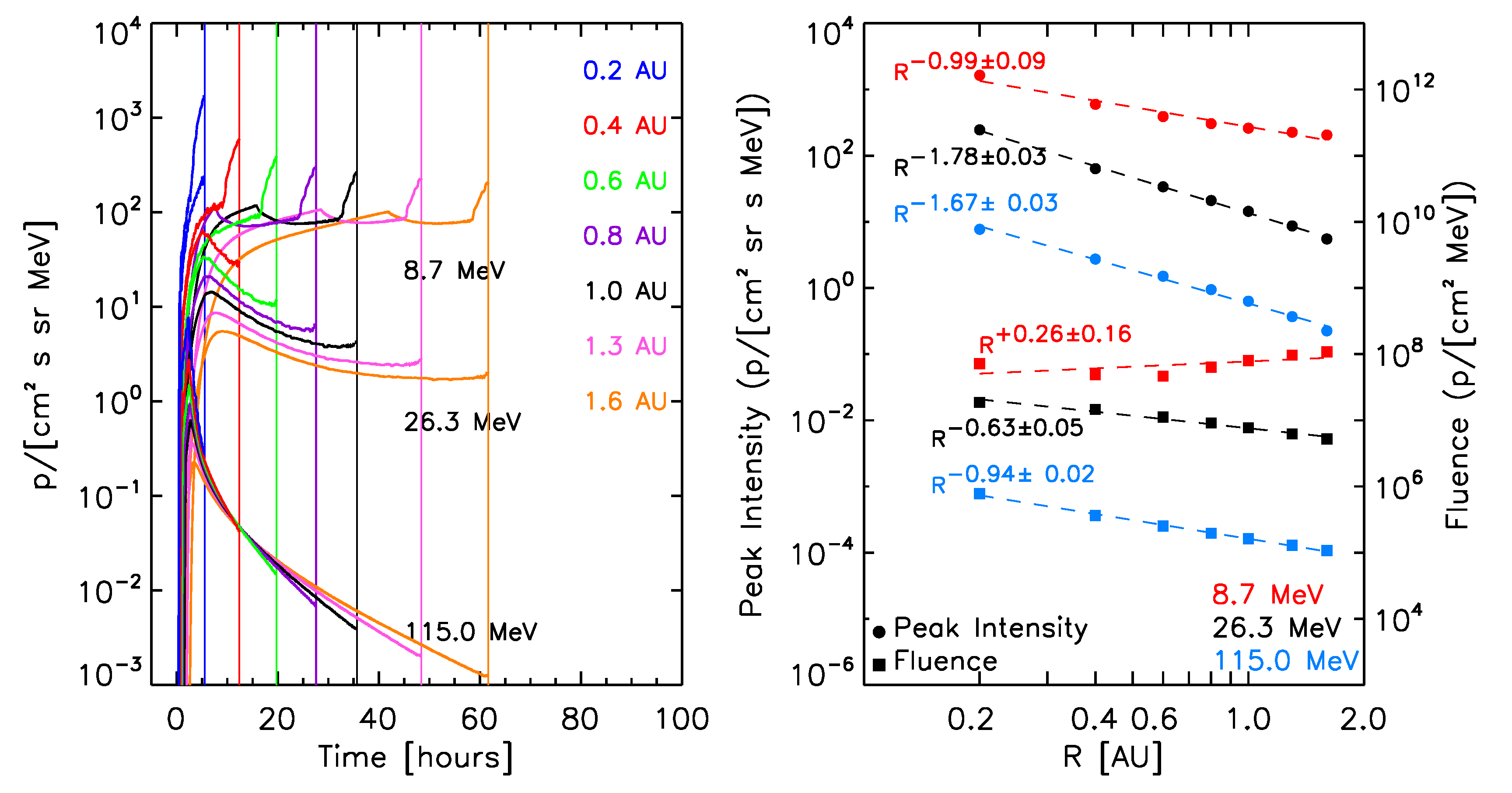

Figure 8. Results of SOLPENCO2 for each reference event. Left panels: Flux profiles at the simulated radial distances for different energies as indicated in each case. Vertical lines mark the time of the shock arrival at each virtual spacecraft. Right panels: Peak intensity (circles) and fluence (squares) variations with the radial distance of the observers. Power-law fits and indices are indicated.

Coupling results from SOLPENCO2 with the SEPEM statistical model

The ultimate goal would be to produce and re-scale synthetic flux profiles using SOLPENCO2 for all SEP events in the REL, in order to reproduce the 1 AU event list at the other six radial distances modelled. Since this represents a rather titanic task, in the mean time, it is possible to use the radial dependences found in the studied events to classify the events in SREL into ten different categories (see below).

The SEP events were classified according to the following characteristics:

presence of an interplanetary shock,
proton intensity enhancements for E>66 MeV,
longitude of the parent solar activity, and
the intensity level reached at the 7.23—10.46 MeV channel (used to determine the initial event list [10]) and, for the largest events in the list, the intensity level reached at the 66.13—95.64 MeV channel.

The main solar eruptions originating the particle events and shock passages at 1 AU were identified for each of the SEP event in the SREL list from January 1988 to April 2013 (249 out of 263 SEP enhancements). Figure 9 shows a screen shot of the event classification.

Proton event list for proton peak intensity and fluence radial dependence — **Figure 9.** Screen shot of the Excel file containing the 249 out of 263 SEP events identified and classified in the January 1988 to April 2013 period. This event list is based on the SEPEM reference data set (RDS) v 2.0 [11].

From the data the following characteristics were determined:

the SEP event start and end time,
the shock arrival times,
the value of the peak intensity,
the up- and downstream fluences and duration,
the X-ray flare and CME (when available) starting times,
the presence of high energy enhancements (hereafter, E>66 MeV)
the intensity reached at 7.23—10.46 MeV (E = 8.7 MeV) and 66.13—95.64 MeV channels (E = 79.5 MeV), and
the solar wind speed.

The SEP events were classified into the following 4 types (10 sub-types):

► Type 1—Events without observed shock

Type 1a. Peak intensity >10 [cm² sr s MeV]^-1 for E=8.7 MeV → Use radial dependences from the 14 December 2006 SEP event.
Type 1b. Peak Intensity <10 [cm² sr s MeV]^-1 for E=8.7 MeV → Use radial dependences determined for the 10 June 2000 SEP event.

► Type 2—Gradual, low-energy cases

A shock is detected in the L1 data and there is no SEP enhancement for E>66 MeV in the upstream region of the SEP events.

Type 2a. Solar origin between W120 and W00 → Use the radial dependences determined from modelling the 4 April 2000 SEP event.
Type 2b. Solar origin between W00 and E45 (both included) → Use the radial dependences from the 6 June 2000 SEP event.
Type 2c. Solar origin between E45 and E90 → Use instead the radial dependences from the 6 March 1989 SEP event.

► Type 3—Gradual, high-energy cases

Type 3a. Peak intensity <50 [cm² sr s MeV]^-1 for E=8.7 MeV and solar origin at or westward from W30 → Use radial dependences from the 13 March 2012 SEP event.
Type 3b. Peak intensity <50 [cm² sr s MeV]^-1 for E=8.7 MeV and solar origin eastward from W30 → Use instead radial dependences determined from the 29 March 2001 SEP event.

► Type 4—Large Gradual, high-energy cases

Type 4a-np. Peak intensity >500 [cm² sr s MeV]^-1 for E=8.7 MeV and >1 [cm² sr s MeV]^-1 for E=79.5 MeV with intensity-time profiles NOT showing a prompt component → Use radial dependences from the 24 September 2001 SEP event.
Type 4a-p. Peak intensity >500 [cm² sr s MeV]^-1 for E=8.7 MeV and >1 [cm² sr s MeV]^-1 for E=79.5 MeV with intensity-time profiles showing a prompt component → Use radial dependences from the 29 October 2003 SEP event.
Type 4b. Peak intensity ≥50 [cm² sr s MeV]^-1 for E=8.7 MeV → Use radial radial dependences determined from the 13 December 2006 SEP event.

The distribution of event sub-types over the events in the SREL is given in the figure and table below.

Number of events per event sub-type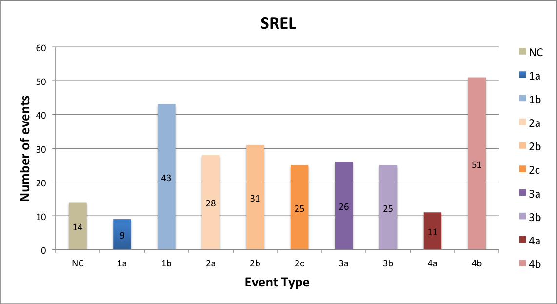

Distribution of event sub-types in the SREL

Event Sub-Type	Fraction in SREL	Event Sub-Type	Fraction in SREL
Type 1a	3%	Type 4a-np	24%
Type 1b	7%	Type 4a-p	24%
Type 2a	29%	Type 4b	10%
Type 2b	21%	Not classified	6%
Type 2c	21%
Type 3a	24%
Type 3b	10%

Figure 10. Number of events in the SREL per sub-type (left) and distribution of event sub-types (right).

The main difference with respect to the former classification of the SEP events is that now we have defined a new type, Type 4, consisting of the larger events (in terms of peak intensity and fluence) in SREL. The Type 4 category is constructed from the previous Type 3a. The two Type 4a categories include the eleven events in SREL with the largest peak intensities at both low and high energy. Further, a new category for Type 2 events has been defined with events associated to far eastern solar sources; and the previous Type 3b category has been split into Type 3 a and b according to the heliolongitude of the associated parent source.

Empirical determination of the fluence in the downstream portion of the SEP events

SOLPENCO2 provides proton intensity-time profiles for the RDS v2.0 differential channels, from the onset of the particle event up to the shock crossing by 1 AU. In order to estimate the fluence in the post-shock region (i.e., the downstream portion of the particle intensity profiles) we have followed an empirical approach.

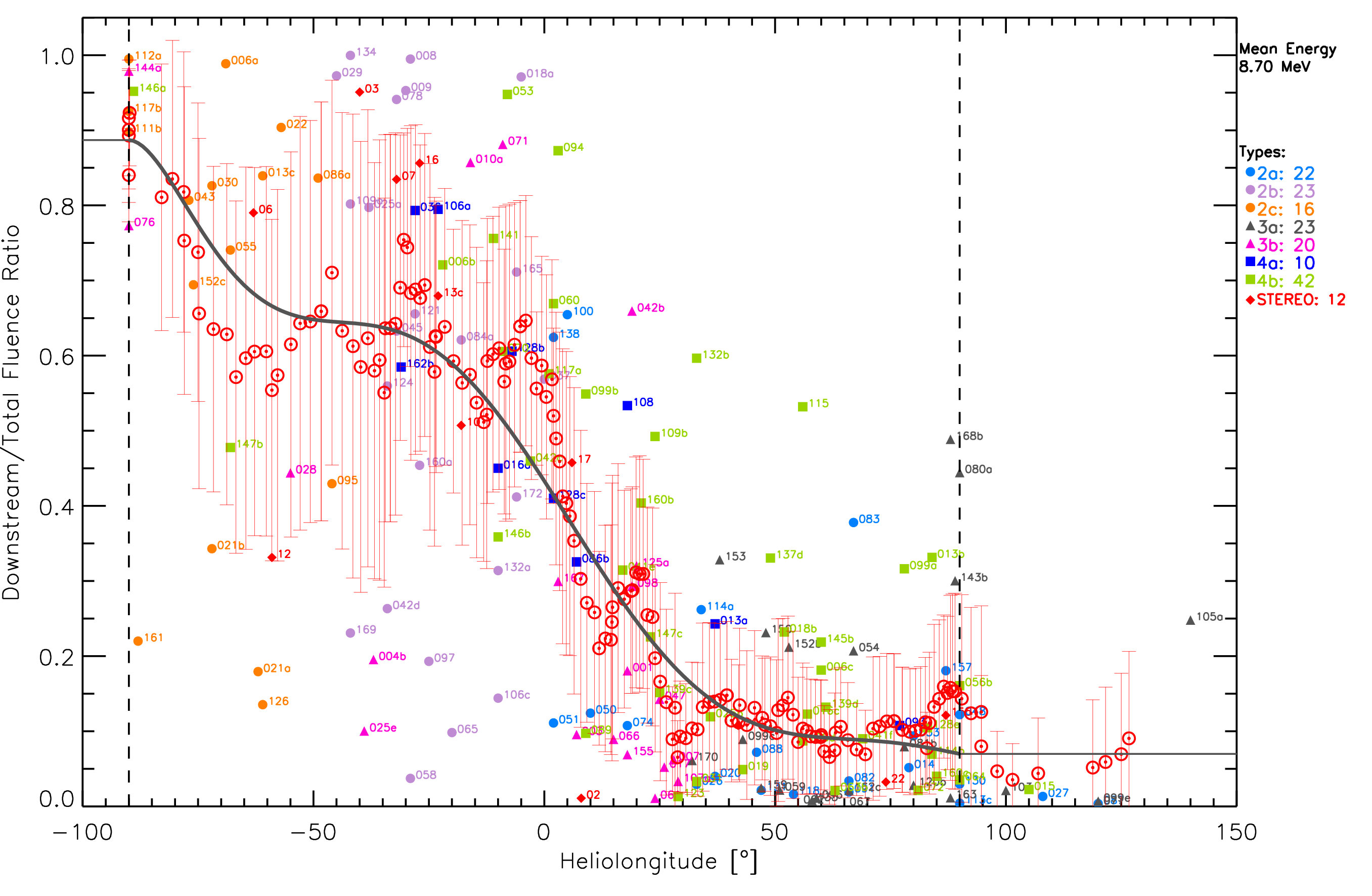
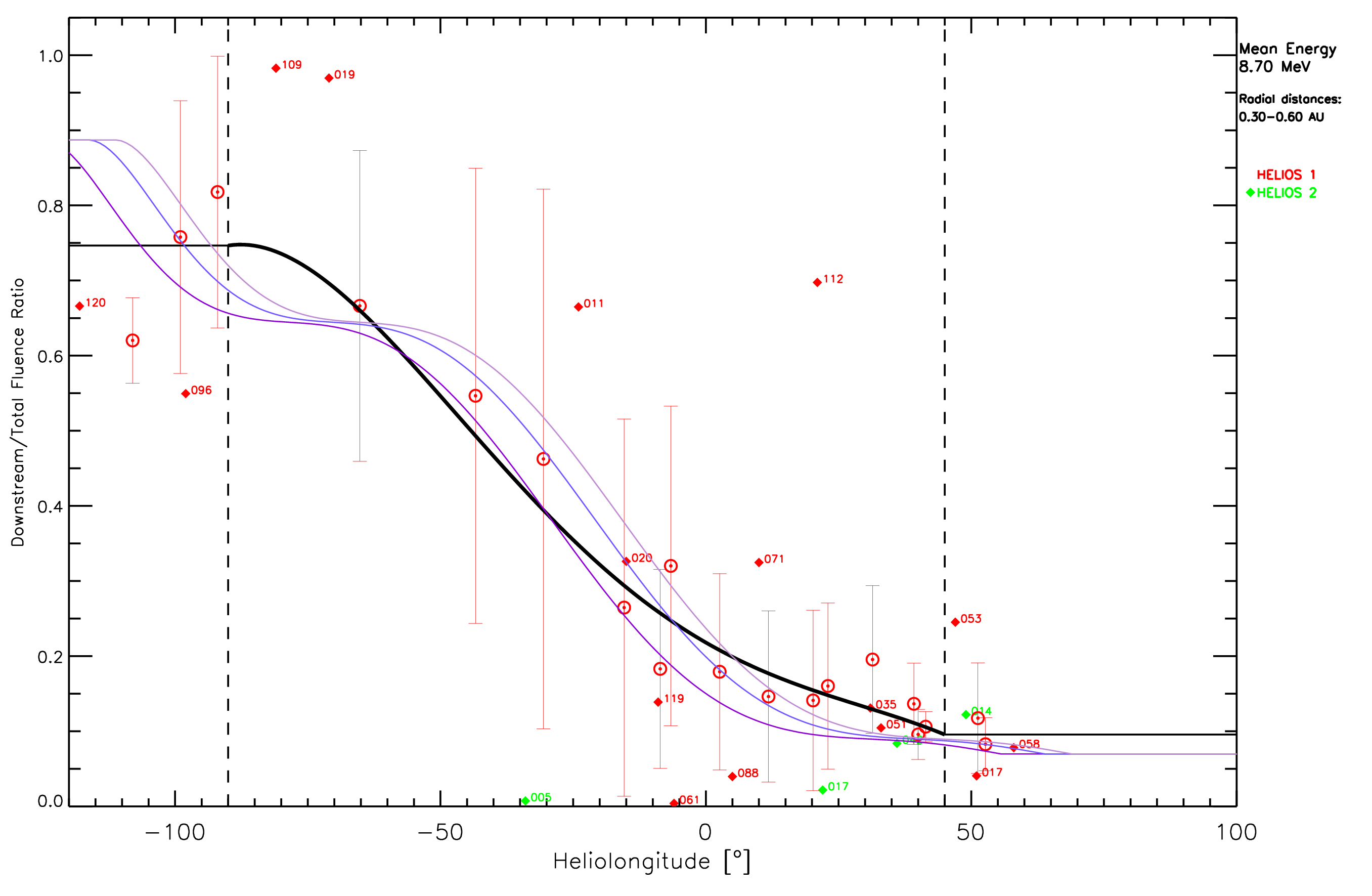
We analysed the 35 SEP events in REL, in the period from January 2007 to April 2013, using multi-spacecraft particle observations from the SEPEM RDS v2.0 and from the STEREO spacecraft. For this study, we selected those events showing (i) a clear association with a main solar source, (ii) intensity-time profiles not significantly affected by other local disturbances at 1 AU, and (iii) the pre-shock and post-shock regions of the intensity-time profiles can be clearly identified. The main conclusion is that in the case of events generated by the same solar eruption there is a variation of the downstream-to-total fluence rations (DTFRs) with the heliolongitude of the parent event: the contribution of the fluence of the downstream region to the total fluence of a given SEP event is larger for the eastern instances of the SEP event than for the western ones [22].

Once it was established that there exists a variation of DTFRs with the heliolongitude in SEP events, we extended the study of the DTFR variation with the heliolongitude to:

the events in the SREL and to their counterparts observed by the twin STEREO spacecraft in order to increase the number of events in the analysis at 1 AU (i.e., 0.96—1.09 AU). The total number of events in this study is 168: 156 from the SREL and 12 from STEREO (see details in [18]).
the events observed away from 1 AU. Here we use the events observed by the Helios spacecraft selected for the downstream analysis and classify these events in two sets depending on the heliocentric radial distance where they were observed: 0.3—0.6 AU (19 SEP events) and 0.6—0.85 AU (22 SEP events).

In summary, from the evaluation of the DTFRs we obtain:

By comparing 6 events simultaneously seen at near-Earth and by one of the STEREO spacecraft, we quantify that the ratios increase toward the eastern locations and decrease with the proton energy [18].
From the analysis of the SEPEM event list and STEREO data, the same tendency is found for the mean values of the DTFRs although the standard deviations derived are high (e.g., see left panel of Figure 11)
From HELIOS data, the small number of events prevents from drawing firm conclusions on the heliocentric radial and longitudinal variation of DTFRs, but indicates that: (i) ratios increase with heliolongitude and (ii) the variation of DTFRs with the heliocentric radial distance are roughly constant for the same angular sector and considering the large standard deviations found.

In order to characterise the DTFRs at other radial distances, we will use the polynomials derived from data at 1 AU, and assume that the longitudinal dependence of the DTFRs is more important than the radial dependence:

The virtual observers away from 1 AU are placed along the same IMF line as the observer at 1 AU (see Figure 1). Therefore, it is possible to translate the longitudinal dependence of the DTFR determined at 1 AU to a radial dependence, by using the angular separation between a given virtual observer away from 1 AU and the observer at 1 AU provided by the bending of the IMF (see details in [22]).
This separation will depend on the solar wind speed detected for each event. In the SREL, the solar wind is classified as `fast', `slow' or `not determined', being the threshold value defining the first two categories, v_sw = 480 km s^-1. In SOLPENCO2 these solar wind scenarios were modelled by taking: v_sw = 365 km s^-1 and v_sw = 595 km s^-1, for the `slow' and `fast' cases respectively [8]. For the `not determined' cases, we have taken the threshold value for the solar wind speed.
Hence, we are assuming that the relative contribution of the downstream portion of the proton intensity-time profiles to the total fluence of SEP events mainly depends on the longitudinal separation of the spacecraft with respect to the direction of the propagation of the associated IP shock.

The right panel of Figure 11 illustrates, for the 8.7 MeV reference energy, the translation of the 1 AU tendencies to the other radial distances. The mauve, violet and purple lines in the right panel of Figure 11 show the grey 1 AU polynomial fit shown in the left panel of this figure, translated to a heliocentric radial distance of r = 0.45 AU, for the three solar wind options. Tendency lines derived for the fast solar wind are the curves with the smallest displacement in longitude (mauve curves) and those for the slow solar wind are the lines showing the largest displacement (purple curve). Tendency lines for the intermediate solar wind lie between the other two (violet curves). The 1 AU derived curves fit closely those derived from the Helios data and, overall, they reside within the standard deviations found for the moving means, apart from one or two points. The same is true for the remaining energy channels, with comparisons at higher energies giving improved results.

Figure 11. DTFRs as a function of the heliolongitude for 8.7 MeV protons. The left panel shows the DTFRs obtained at 1 AU as a function of the heliolongitude for the events in SREL (labels indicate the event number) plus the STEREO events for which the DTFRs could be calculated. The red open circles are the moving means obtained with a window of 11 points and the bars indicate the standard deviation of the data points in the running window. The dependence of DTFRs with the heliolongitude is defined by polynomial fits to the moving means (grey solid line). The right panel shows the DTFRs for events detected at 0.3—0.6 AU (labels indicate the event number). Red open circles and bars correspond to the moving mean (of 7 points) values and standard deviations. The black thick line between -90° to 90° corresponds to a polynomial fit applied to the mean DTFR values. Tendency lines derived from 1 AU data for the three solar wind speeds are shown for comparison: mauve lines correspond to the fast solar wind case, violet lines to the intermediate solar wind speed, and purple lines to the slow solar wind.

In conclusion, we use the polynomial fits derived from 1 AU to characterise the variation of the DTFRs for the virtual observers located away from 1 AU. In the implementation of these results into the total fluence computation of the SREL events away from 1 AU, we vertically translate the tendency curve found to match the observed DTFR value at 1 AU for each event, and then we apply the corresponding angular displacement, following the general tendency curves derived. That is, we assume that the polynomial fits derived represent the "Average Variation" with heliolongitude, and apply the same tendency for all events, starting from the observed DTFR value at the observed heliolongitude. As an example, Figure 12 shows the radial dependence of the upstream (directly from SOPENCO2) and total fluence (after determining the downstream fluence variation) for two of the reference events which showed upstream fluence increasing with helioradial distance. The method for deriving the total fluence has reduced this by assigning greater downstream fluence to the lower helioradial distance observers, especially at lower energies.

**Figure 12.** Radial dependence of the upstream fluence (left panels) and total fluence (right panels) for three different proton energies, 6.01 MeV (orange), 18.18 MeV (blue) and 79.53 MeV (purple) for the Type 2c reference case (left set) and the Type 4a-np reference case (right set).
Type 2c. 1989 March 6 SEP event.	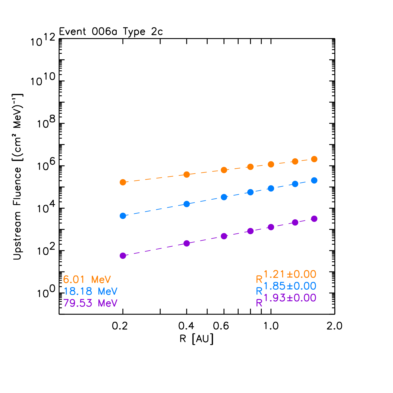	Type 4a-np. 2001 September 24 SEP event.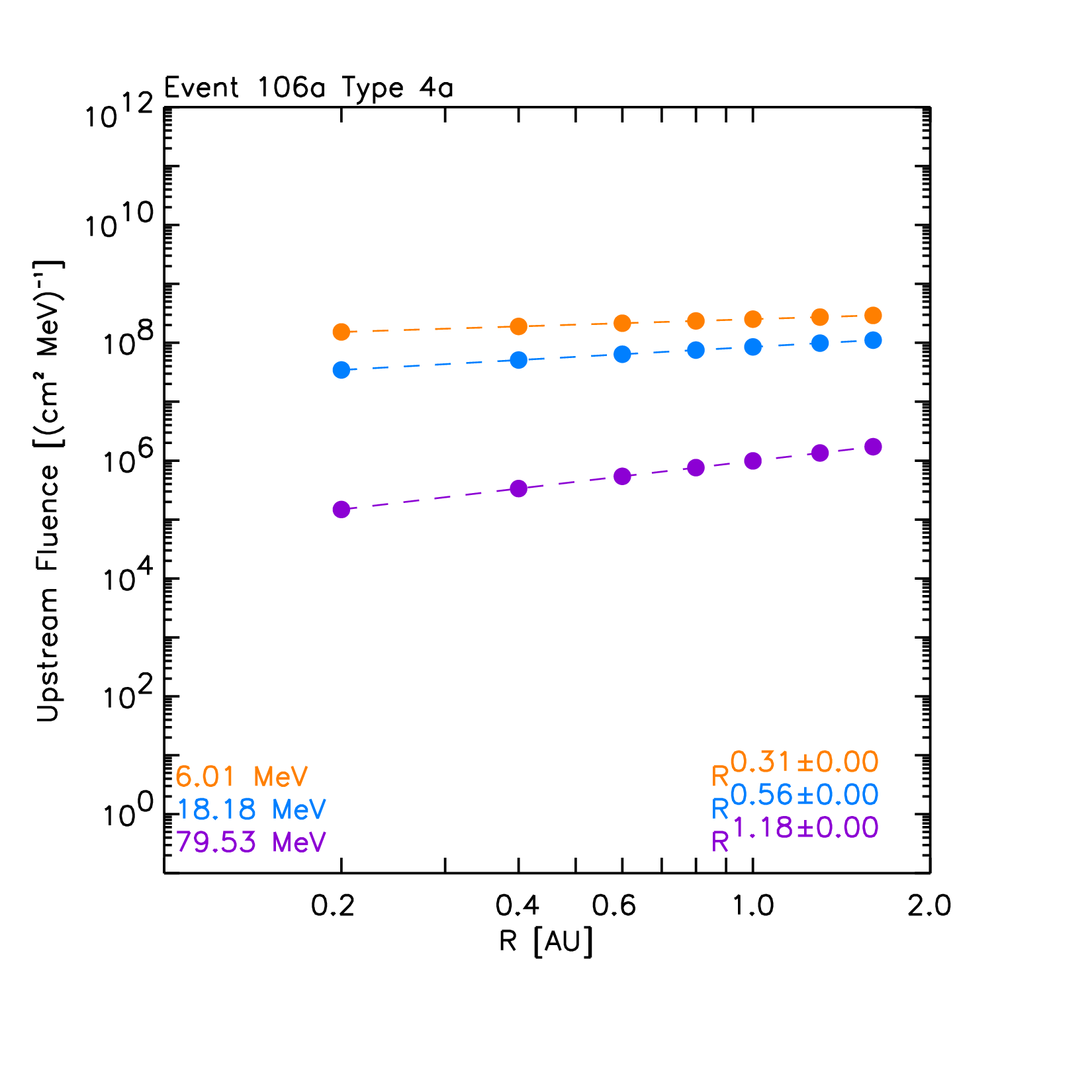

Determination of the radial dependencies for all events in SREL

Once the SEP events in REL are classified into one of the ten sub-types, the peak intensity and fluence spectra across radial distances can be computed. Figure 13 shows an example of the resulting spectra for the individual SEP event on 13 May 2005. After revision of the data set, this event was classified as a Type 4b event. The left panel of Figure 13 shows the peak intensity energy spectra across the simulated radial distances (colour coded) whereas the right panel shows the corresponding plot for the total fluence. The largest values are obtained for the virtual observer located at 0.2 AU, with the exception of the fluence for the two lower energies. In these latter cases, the predicted heliocentric radial dependence of the fluence is almost flat, resulting from the radial dependence derived by SOLPENCO2 for the 2006 December 13 SEP event (the reference event for Type 4b) for these two energies.

Figure 13. Peak intensity (left) and fluence (right) spectra of the 13 May 2005 SEP event for each modelled radial distance (colour coded as indicated in the legends). SEPEM RDS used is v2.0 with background subtraction described in [22].

In compound SEP events, the downstream region of one event is overlapped by the onset of the following event. The contributions of any remaining flux resulting from the first shock or from re-acceleration by the following shock are included in the later event. The method has little background physical support. It is aimed to give an operative input for the statistical model.

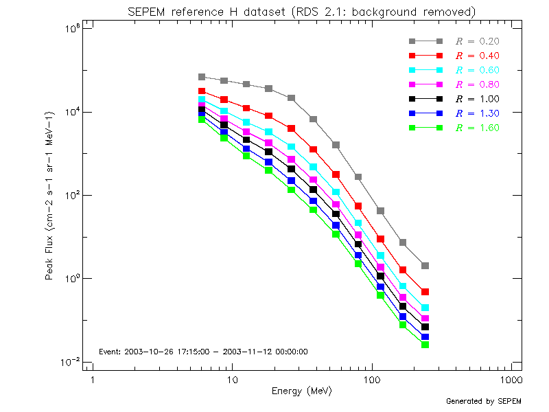
In such compound events, the peak intensity of each proton enhancement has been scaled to other radial distances according to its sub-type and the selected value is the highest among the SEP enhancements for each energy and radial distance. To compute the fluences of the compound events, first the fluence of each individual SEP event (or each SEP enhancement) is scaled according to the power law of its sub-type. Next, the scaled fluences are added to account for the fluence of the compound event. Figure 14 shows the example of the Halloween events in October—November 2003. This compound event is formed by 5 SEP events, two of them classified as Type 4a-p and the other three as Type 4b. As in the previous figure, Figure 14 shows the peak intensity (left) and total fluence (right) energy spectra across the simulated radial distances (colour coded) for the Halloween events. For both magnitudes and for all energies, the largest values are predicted for the virtual observer placed at the closest distance from the Sun.

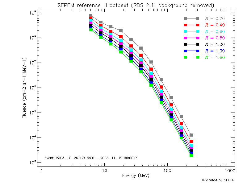Figure 14. Intensity spectra for the Halloween events (26 October—12 November 2003) using SEPEM RDS v2.1

Away from 1 AU analysis

The specific method used to include the radial dependent information into the statistical modelling may be outlined as follows:

The total mission period is divided up into successive segments of solar maximum and solar minimum periods, using 7 and 4 year windows around solar maximum (2.5 years before solar maximum to 4.5 years after) and solar minimum, respectively. For missions in the future, the current solar maximum date is repeated with an 11 year cycle.
After a sampled waiting time an SEP event is generated with an associated duration as if the spacecraft were at 1 AU.
The fluence/peak flux of the events is scaled for the spacecraft orbital position at that instance.
This fluence/peak flux is recorded, the next waiting time is generated, the next event size found and scaled, and then added to the total (or compared to the running maximum flux).
This procedure is repeated until the virtual timeline reaches the planned mission end.
The whole process is repeated for 100,000 iterations, for the current solar cycle phase, and the results are stored.
When all solar cycle phase segments have been processed, the results for the individual segments are accumulated.

Future work

We have presented a methodology (in fact, the first attempt ever) to couple physics-based models, considering the description of gradual SEP events, with statistical SEP environment models, in order to address the variation of the peak intensities and fluence of SEP events for interplanetary missions travelling in the inner heliosphere. The present results may be ameliorated by improving both the SOLPENCO2 tool and the physics-based shock-and-particle (SaP) model described above [8]. In particular, future developments could include (but not only):

Model more events with the present version of the SaP model (i.e., [9]) in order to derive semi-empirical relations between the injection rate of escaping protons from the shock, Q, and the VR parameter, and in this way, extend the number of modelled cases (presently only the 2000 April 4 event and the 2006 December 13 event).
Replace the data base of IP shocks done for SEPEM with a similar data base of shock run with the 2D MHD developed by [9] due to its better simulation of the solar wind. In spite of this being a 2D MHD model, it has the advantage that it starts from low in the corona.
Model magnetic connections other than the nominal Parker IMF, and in case shock-acceleration models results allow for it, improve the modelling of the foreshock region.
Model with SOLPENCO2 the larger 11 SEP events of Type 4a plus the 2005 January 20 SEP event (the event with the harder spectrum for > 10 MeV). And split the most populated category, the Type 4b events, into different sub-types, e.g., considering the relative longitude between the observers and the solar source.
Use the potential grid of synthetic profiles of SOLPENCO2 to finally have a statistical model based on synthetic profiles, where the downstream portion could be somehow modelled to provide a full synthetic time series of events.
More SEP events should be modelled, considering also non-ideal configurations, as for example, the effect of intervening structures to enhance SEP intensities [23].

The Solar Orbiter and the Parker Solar Probe missions may help to improve and verify our models.

The work presented here is documented in a series of internal ESA/SEPEM Technical Reports. Part of these results is still in the process of publication.

References

[1] Aran A., B. Sanahuja and D. Lario (2006) Advances in Space Research 37, 1240.

[2] Aran A., B. Sanahuja and D. Lario (2005) Annales Geophysicae 23, 3047.

[3] Aran, A., PhD Thesis, (2007).

[4] Wu, S. T., M. Dryer and S. M. Han (1983) Solar Phys. 84, 395.

[5] Lario D., B. Sanahuja, and A.M. Heras (1998) Astrophys. Journal 509, 415.

[6] Aran A., B. Sanahuja and D. Lario (2008), Advances in Space Research, 42(9), 1492-1499, doi:10.1016/j.asr.2007.08.003

[7] Crosby, N., D. Heynderickx, P. Jiggens et al. (2015), Space Weather, 13, 406-426, doi:10.1002/2013SW001008

[8] Aran, A., C. Jacobs, R. Rodríguez-Gasén et al. (2011). WP410: Initial and boundary conditions for the shock-and- particle model. SEPEM Technical Report, ESA/ESTEC Contract 20162/06/NL/JD, 1–58.

[9] Pomoell, J., A. Aran, C. Jacobs et al. (2015) , Journal of Space Weather and Space Climate, 5, A12, doi:10.1051/swsc/201505.

[10] Jiggens. P., S. Gabriel, D. Heynderickx, et al. (2012), IEEE Trans. Nuc. Sci., 59(4), 1066.

[11] Sandberg, I., (2014), SEPCALIB Final Report, 1-40.

[12] Cane H.V. and D. Lario, (2006), Space Science Reviews, 123, 45-56.

[13] Jacobs C. and S. Poedts (2011), Advances in Space Research, 48, 1958.

[14] A. M. Heras, B. Sanahuja, Z. Smith et al. (1992), Astrophys. Journal 391, 359

[15] A.M. Heras, B. Sanahuja, D. Lario et al. (1995), Astrophys. Journal 445, 497.

[16] E. C. Roelof (1969), in Lectures in High Energy Astrophysics, NASA SP-199, ed. H. Ögelman & J. R. Wayland, 111.

[17] D. Ruffolo (1995), Astrophys. Journal, 442, 861.

[18] J. R. Jokipii (1966) Astrophys. Journal 146, 480.

[19] A. Aran et al. (2007) Astron. & Astrophys. 469, 1123.

[20] D. Lario, M.-B. Kallenrode, et al (2006) Astrophys. Journal 653, 1531

[21] D. Lario, A. Aran et al. (2007) Advances in Space Research 40, 289.

[22] Pacheco, D., A. Aran, N. Agueda, B. Sanahuja (2017), SOL2UP WP1200: Evaluation of the downstream contribution to total fluence, SOL2UP Technical Report TN-1, ESA/ESTEC contract 4000114116/15/NL/HK, 1—134 (2017); Pacheco et al., JSWSC in preparation (2017).

[23] Lario, D., A. Aran, R. Gómez-Herrero, et al. (2013), Astrophys. J., 767, 41.

Last modified: July 2017